Chapter 2 Exploration Diagnostic

2.1 Setup

First, we need to do some set up to analyze our data

Include dependencies

library(ggplot2)       # For plotting
library(tidyverse)     # For data wrangling
library(knitr)         # For making nice rmarkdown documents
library(cowplot)       # For theme
library(viridis)       # For color scale
library(RColorBrewer)  # For more color scales
library(rstatix)
library(ggsignif)      # For adding pairwise significance to plots
library(Hmisc)         # For bootstrapping condifence internvals
library(kableExtra)    # For displaying nice tables
source("https://gist.githubusercontent.com/benmarwick/2a1bb0133ff568cbe28d/raw/fb53bd97121f7f9ce947837ef1a4c65a73bffb3f/geom_flat_violin.R") # For raincloud plots
library(readr)        # For reading in data
library(stringr)      # For manipulating string data
library(ggpubr)       # For displaying correlation statistics on plots
library(infotheo)     # For causality analysis
library(scales)       # For displaying scales nicely in facetted plots
library(osfr)         # For downloading the data for this project

These analyses were conducted in the following computing environment:

print(version)

##                _                           
## platform       x86_64-apple-darwin17.0     
## arch           x86_64                      
## os             darwin17.0                  
## system         x86_64, darwin17.0          
## status                                     
## major          4                           
## minor          1.1                         
## year           2021                        
## month          08                          
## day            10                          
## svn rev        80725                       
## language       R                           
## version.string R version 4.1.1 (2021-08-10)
## nickname       Kick Things

Setup constants to be used across plots

# Labeler for stats annotations
p_label <- function(p_value) {
  threshold = 0.0001
  if (p_value < threshold) {
    return(paste0("p < ", threshold))
  } else {
    return(paste0("p = ", p_value))
  }
}

# Significance threshold
alpha <- 0.05

# Common graph variables
performance_ylim <- 1
coverage_ylim <- 1.0

####### misc #######
# Configure our default graphing theme
theme_set(theme_cowplot())

The data for this project are hosted on osf.io. The following chunk downloads them automatically if they haven’t already been downloaded.

# Read in data
osf_retrieve_file("esm4r") %>% osf_download(conflicts = "skip")  # Download data from osf
data_loc <- "final_exploration_diagnostic_data.csv"

data <- read_csv(data_loc, na=c("NONE", "NA", ""))

## Clean up data columns

# Make selection name column human readable
data <- data %>% mutate(selection_name = as.factor(case_when(
  selection_name == "EpsilonLexicase" ~ "Lexicase",
  TOUR_SIZE == 1 ~ "Random",
  selection_name == "Tournament" ~ "Tournament",
  selection_name == "FitnessSharing" ~ "Fitness Sharing",
  selection_name == "EcoEa" ~ "EcoEA"
)))

# Calculate performance statistics.
# Elite trait avg is the avg per-site performance of the best individual
data$elite_trait_avg <-
  data$ele_agg_per / data$OBJECTIVE_CNT
data$unique_start_positions_coverage <-
  data$uni_str_pos / data$OBJECTIVE_CNT

# Convert elite_trait_avg to percent of maximum possible
data$elite_trait_avg <- data$elite_trait_avg/data$TARGET

# Grab data from just the final time point
final_data <- filter(data, evaluations==max(data$evaluations))

2.2 Performance

For context, it’s important to know how each selection scheme performed on the exploration diagnostic.

2.2.1 Over time

First we look at the dynamics of performance over time.

2.2.1.1 Trait performance

Here, we plot average trait performance (i.e. fitness) over time for each selection scheme. We log the x-axis because Eco-EA gains fitness over a very long time scale, whereas the interesting dynamics for the other selection schemes occur relatively quickly.

ggplot(
    data,
    aes(
      x=gen,                 # Generations
      y=elite_trait_avg,     # Performance
      color=selection_name,  # Selection scheme
      fill=selection_name
    )
  ) +
  stat_summary(geom="line", fun=mean) + # Plot line showing mean for each selection scheme
  stat_summary(  # Add shading around each line indicating 95% confiedence interval
    geom="ribbon",
    fun.data="mean_cl_boot",
    fun.args=list(conf.int=0.95),
    alpha=0.2,
    linetype=0
  ) +
  scale_y_continuous(
    name="Average trait performance", # Set y axis title
    limits=c(0, performance_ylim)  # Set y axis range to include all possible performance values
  ) +
  scale_x_log10(  # Log x axis
    name="Generation" # Set x axis title
  ) +
  scale_color_discrete("Selection") + # Set legend title
  scale_fill_discrete("Selection")    # Set legend title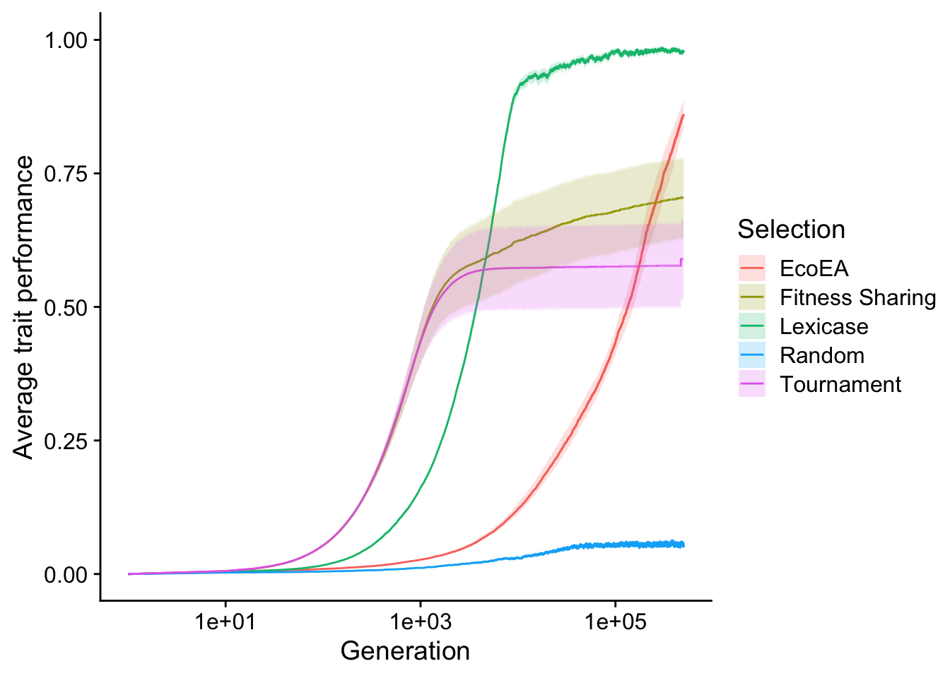

As observed by Hernandez et al. in their original paper on the exploration diagnostic (Hernandez, Lalejini, and Ofria 2021), fitness in tournament selection initially increases quickly and then plateaus. Fitness in lexicase selection increases slightly slower but plateaus at a much higher value (nearly 100%). Fitness sharing behaves similarly to tournament selection, but maintains a slight upward trajectory (note that, because the x axis is on a log scale, this trajectory is very gradual). Eco-EA takes substantially longer to increase in fitness but ultimately surpasses fitness sharing and tournament selection. It is unclear whether it would pass lexicase selection if these runs were allowed to continue for slightly longer; they do not appear to have plateaued yet. We chose to cut them off at 500,000 generations due to resource constraints and the fact that the questions we’re asking here are not really about final fitness.

2.2.1.2 Activation position coverage

Out of curiosity, we also ran the analysis of unique activation positions present in the population, used by Hernandez et. al. This analysis tells us about the diversity of start positions for the coding region represented in the population. As the set of start positions in the population tends to represent a meaningful constraint on the number of paths through the fitness landscape that are currently accessible, this is in some sense a metric of useful diversity in the population

ggplot(data, aes(x=gen, y=unique_start_positions_coverage, color=selection_name, fill=selection_name)) +
  stat_summary(geom="line", fun=mean) +
  stat_summary(
    geom="ribbon",
    fun.data="mean_cl_boot",
    fun.args=list(conf.int=0.95),
    alpha=0.2,
    linetype=0
  ) +
  scale_y_continuous(
    name="Activation position coverage"
  ) +
  scale_x_log10(
    name="Generation"
  ) +
  scale_color_discrete("Selection")+
  scale_fill_discrete("Selection")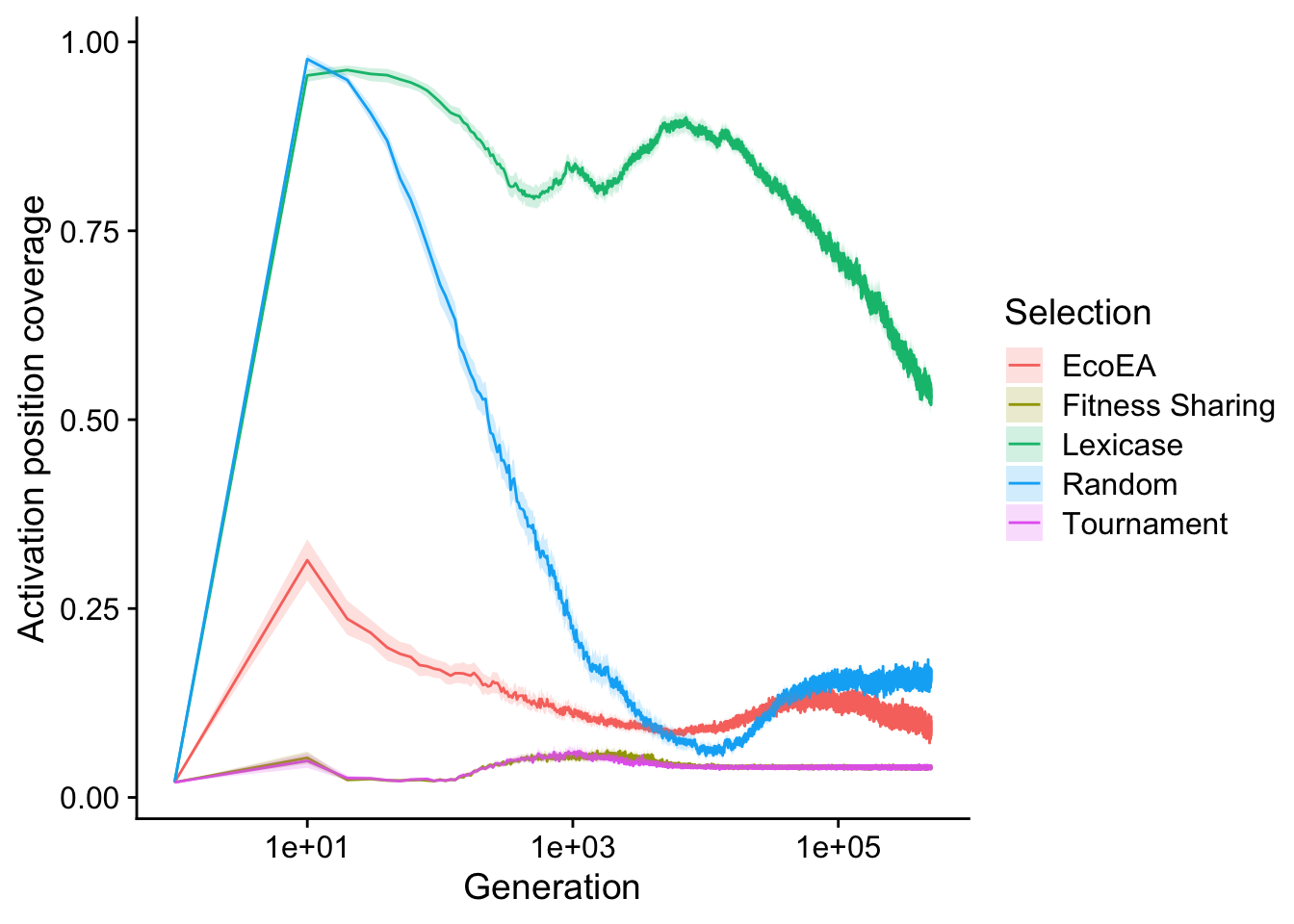

We see that lexicase selection maintains by far that largest number of unique start positions, even surpassing the number maintained by random drift. This suggests that lexicase selection is actively selecting for maintaining a diversity of start positions. Tournament selection and fitness sharing perform virtually identically, with Eco-EA falling in between.

2.2.2 Final

While trends over time are more informative, it can be hard to visualize the full distribution (particularly the extent of variation). Thus, we also conduct a more detailed analysis of performance at the final time point.

2.2.2.1 Trait performance

First we conduct statistics to identify which selection schemes are significantly different from each other.

# Compute manual labels for geom_signif
stat.test <- final_data %>%
  wilcox_test(elite_trait_avg ~ selection_name) %>%
  adjust_pvalue(method = "bonferroni") %>%  # Apply Bonferroni correction for multiple comparisons
  add_significance() %>%
  add_xy_position(x="selection_name",step.increase=1)
stat.test$label <- mapply(p_label,stat.test$p.adj)

Then we make raincloud plots (Allen et al. 2021) of each selection scheme.

elite_final_performance_fig <- ggplot(
    final_data,
    aes(
      x=selection_name,
      y=elite_trait_avg,
      fill=selection_name
    )
  ) +
  geom_flat_violin(
    position = position_nudge(x = .2, y = 0),
    alpha = .8,
    scale="width"
  ) +
  geom_point(
    mapping=aes(color=selection_name),
    position = position_jitter(width = .15),
    size = .5,
    alpha = 0.8
  ) +
  geom_boxplot(
    width = .1,
    outlier.shape = NA,
    alpha = 0.5
  ) +
  scale_y_continuous(
    name="Average trait performance",
    limits=c(0, performance_ylim)
  ) +
  scale_x_discrete(
    name="Selection"
  ) +
  scale_fill_discrete(
    name="Selection"
  ) +
  scale_color_discrete(
    name="Selection"
  ) + 
  theme(legend.position="none")
elite_final_performance_fig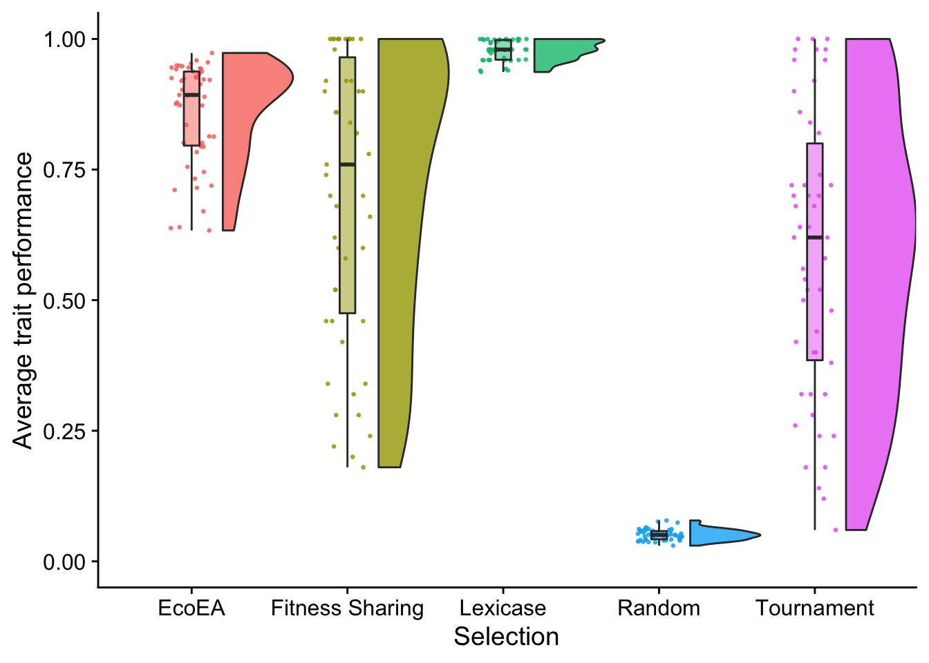

These observations look fairly consistent with the timeseries plots.

Next, we output the results of our significance testing.

stat.test %>%
  kbl() %>%
  kable_styling(
    bootstrap_options = c(
      "striped",
      "hover",
      "condensed",
      "responsive"
    )
  ) %>%
  scroll_box(width="600px")

.y.	group1	group2	n1	n2	statistic	p	p.adj	p.adj.signif	y.position	groups	xmin	xmax	label
elite_trait_avg	EcoEA	Fitness Sharing	50	50	1561	3.20e-02	3.20e-01	ns	1.922000	EcoEA , Fitness Sharing	1	2	p = 0.32
elite_trait_avg	EcoEA	Lexicase	50	47	60	0.00e+00	0.00e+00	****	2.946444	EcoEA , Lexicase	1	3	p < 1e-04
elite_trait_avg	EcoEA	Random	50	50	2500	0.00e+00	0.00e+00	****	3.970889	EcoEA , Random	1	4	p < 1e-04
elite_trait_avg	EcoEA	Tournament	50	50	1939	2.10e-06	2.07e-05	****	4.995333	EcoEA , Tournament	1	5	p < 1e-04
elite_trait_avg	Fitness Sharing	Lexicase	50	47	593	2.69e-05	2.69e-04	***	6.019778	Fitness Sharing, Lexicase	2	3	p = 0.000269
elite_trait_avg	Fitness Sharing	Random	50	50	2500	0.00e+00	0.00e+00	****	7.044222	Fitness Sharing, Random	2	4	p < 1e-04
elite_trait_avg	Fitness Sharing	Tournament	50	50	1549	4.00e-02	4.00e-01	ns	8.068667	Fitness Sharing, Tournament	2	5	p = 0.4
elite_trait_avg	Lexicase	Random	47	50	2350	0.00e+00	0.00e+00	****	9.093111	Lexicase, Random	3	4	p < 1e-04
elite_trait_avg	Lexicase	Tournament	47	50	2098	0.00e+00	0.00e+00	****	10.117556	Lexicase , Tournament	3	5	p < 1e-04
elite_trait_avg	Random	Tournament	50	50	10	0.00e+00	0.00e+00	****	11.142000	Random , Tournament	4	5	p < 1e-04

Fitness sharing did not perform significantly differently from Eco-EA or Tournament selection, but all other selection schemes are significantly different.

2.2.2.2 Final activation position Coverage

Now we do the same analysis for final activation position coverage.

First we calculate the statistics

# Compute manual labels for geom_signif
stat.test <- final_data %>%
  wilcox_test(unique_start_positions_coverage ~ selection_name) %>%
  adjust_pvalue(method = "bonferroni") %>%
  add_significance() %>%
  add_xy_position(x="selection_name",step.increase=1)
stat.test$manual_position <- stat.test$y.position * 1.05
stat.test$label <- mapply(p_label,stat.test$p.adj)

Then we make raincloud plots

unique_start_positions_coverage_final_fig <- ggplot(
    final_data,
    aes(
      x=selection_name,
      y=unique_start_positions_coverage,
      fill=selection_name
    )
  ) +
  geom_flat_violin(
    position = position_nudge(x = .2, y = 0),
    alpha = .8,
    scale="width"
  ) +
  geom_point(
    mapping=aes(color=selection_name),
    position = position_jitter(width = .15),
    size = .5,
    alpha = 0.8
  ) +
  geom_boxplot(
    width = .1,
    outlier.shape = NA,
    alpha = 0.5
  ) +
  scale_y_continuous(
    name="Activation position coverage",
    limits=c(0, coverage_ylim)
  ) +
  scale_x_discrete(
    name="Selection"
  ) +
  scale_fill_discrete(
    name="Selection"
  ) +
  scale_color_discrete(
    name="Selection"
  ) +
  theme(
    legend.position="none"
  )
unique_start_positions_coverage_final_fig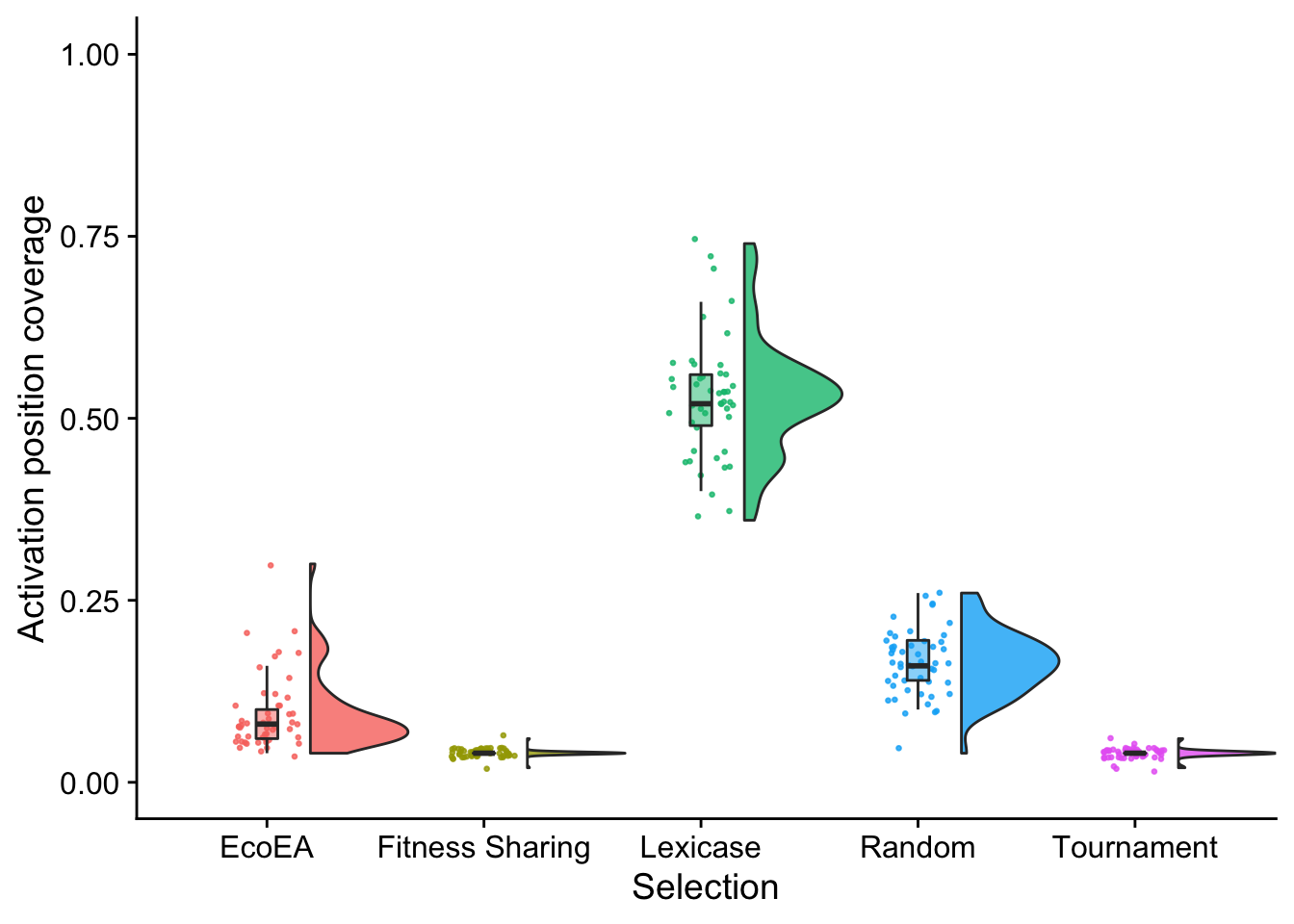

These also look unsurprising.

Lastly, we output the results of significance testing.

stat.test %>%
  kbl() %>%
  kable_styling(
    bootstrap_options = c(
      "striped",
      "hover",
      "condensed",
      "responsive"
    )
  ) %>%
  scroll_box(width="600px")

.y.	group1	group2	n1	n2	statistic	p	p.adj	p.adj.signif	y.position	groups	xmin	xmax	manual_position	label
unique_start_positions_coverage	EcoEA	Fitness Sharing	50	50	2392.5	0.000	0	****	1.420000	EcoEA , Fitness Sharing	1	2	1.491000	p < 1e-04
unique_start_positions_coverage	EcoEA	Lexicase	50	47	0.0	0.000	0	****	2.175556	EcoEA , Lexicase	1	3	2.284333	p < 1e-04
unique_start_positions_coverage	EcoEA	Random	50	50	339.0	0.000	0	****	2.931111	EcoEA , Random	1	4	3.077667	p < 1e-04
unique_start_positions_coverage	EcoEA	Tournament	50	50	2387.0	0.000	0	****	3.686667	EcoEA , Tournament	1	5	3.871000	p < 1e-04
unique_start_positions_coverage	Fitness Sharing	Lexicase	50	47	0.0	0.000	0	****	4.442222	Fitness Sharing, Lexicase	2	3	4.664333	p < 1e-04
unique_start_positions_coverage	Fitness Sharing	Random	50	50	25.0	0.000	0	****	5.197778	Fitness Sharing, Random	2	4	5.457667	p < 1e-04
unique_start_positions_coverage	Fitness Sharing	Tournament	50	50	1274.5	0.708	1	ns	5.953333	Fitness Sharing, Tournament	2	5	6.251000	p = 1
unique_start_positions_coverage	Lexicase	Random	47	50	2350.0	0.000	0	****	6.708889	Lexicase, Random	3	4	7.044333	p < 1e-04
unique_start_positions_coverage	Lexicase	Tournament	47	50	2350.0	0.000	0	****	7.464444	Lexicase , Tournament	3	5	7.837667	p < 1e-04
unique_start_positions_coverage	Random	Tournament	50	50	2475.5	0.000	0	****	8.220000	Random , Tournament	4	5	8.631000	p < 1e-04

2.3 Phylogenetic diversity

Next, we analyze the behavior of phylogenetic diversity on the exploration diagnostic.

2.3.1 Relationship between different types of pylogenetic diversity

First, to get a big-picture overview, we make correlation matrices of all the different phylogenetic diversity metrics:

final_data %>% 
  transmute(MinPD=min_phenotype_pairwise_distance, 
            MeanPD=mean_phenotype_pairwise_distance, 
            MaxPD=max_phenotype_pairwise_distance, 
            VarPD=variance_phenotype_pairwise_distance, 
            MinED = min_phenotype_evolutionary_distinctiveness,
            MeanED= mean_phenotype_evolutionary_distinctiveness,
            MaxED=max_phenotype_evolutionary_distinctiveness,
            VarED=variance_phenotype_evolutionary_distinctiveness,
            PD=phenotype_current_phylogenetic_diversity,  # See Faith 1992
            MRCA=phen_mrca_depth,  # Phylogenetic depth of most recent common ancestor
            N=phen_num_taxa     # Number of taxonomically-distinct phenotypes
  ) %>%
  cor_mat() %>% 
  pull_lower_triangle() %>% 
  cor_plot()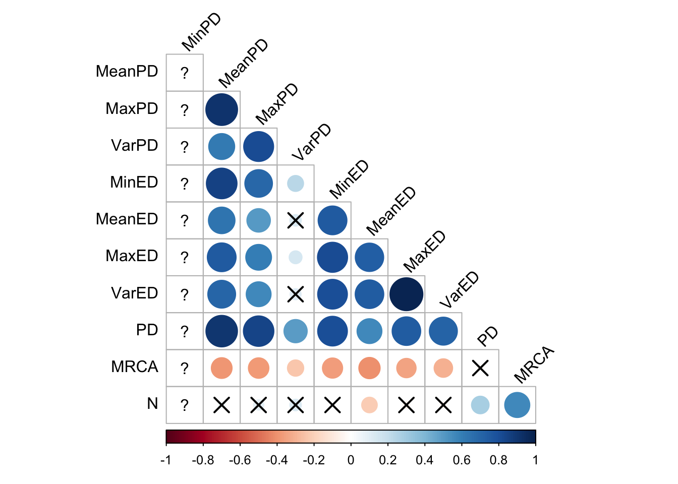

However, these correlations may well vary by selection scheme, and even over time within a selection scheme. Let’s take a look at some scatter plots.

ggplot(
    data %>% filter(gen==500000),
    aes(
        y=mean_phenotype_pairwise_distance,
        x=variance_phenotype_pairwise_distance,
        color=selection_name,
        fill=selection_name
    )
  ) +
  geom_point() +
  scale_x_continuous(
        breaks = breaks_extended(4)
  ) + 
  facet_wrap(
      ~selection_name, scales="free"
  ) + 
  stat_smooth(
    method="lm"
  ) + 
  stat_cor(
    method="spearman", cor.coef.name = "rho", color="black"
  ) +
  theme(legend.position = "none")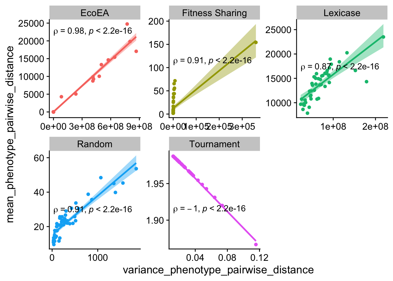

Mean and variance of pairwise distances appears to correlate fairly closely with each other across selection schemes. The exception to this is tournament selection, where the range of values for both of these metrics are very small and the correlation is directly inverse. This is likely being driven by there being a small number of taxa that are mostly siblings of each other.

ggplot(
    data %>% filter(gen==500000),
    aes(
        y=mean_phenotype_pairwise_distance,
        x=max_phenotype_pairwise_distance,
        color=selection_name,
        fill=selection_name
    )
  ) +
  geom_point() +
  scale_x_continuous(
        breaks = breaks_extended(4)
  ) + 
  facet_wrap(
      ~selection_name, scales="free"
  ) + 
  stat_smooth(
    method="lm"
  ) + 
  stat_cor(
    method="spearman", cor.coef.name = "rho", color="black"
  ) +
  theme(legend.position = "none")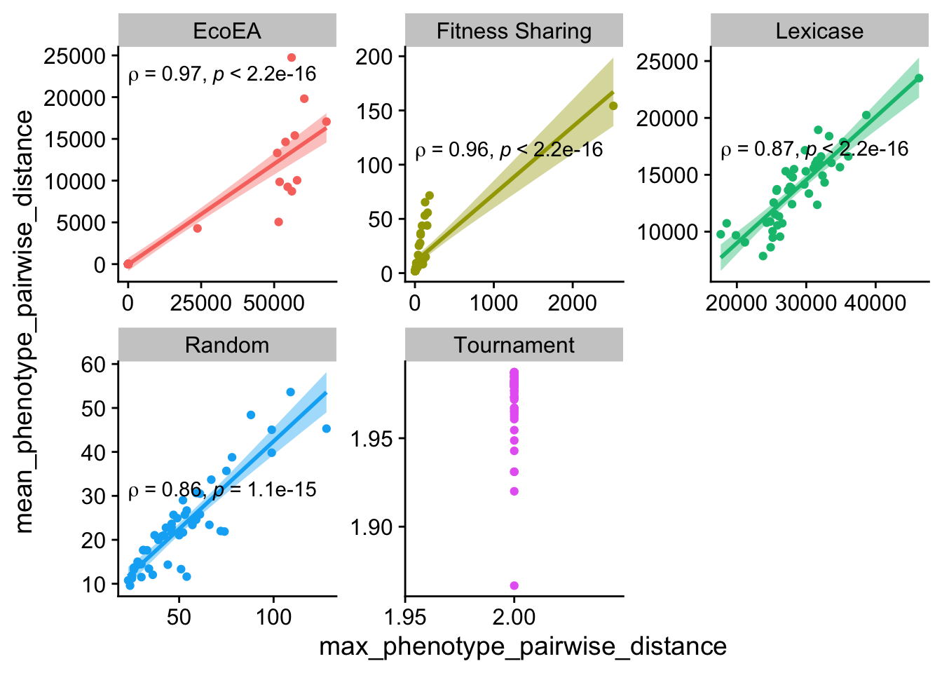

Maximum and mean pairwise distance also correlate pretty closely, with the exception again being tournament. These data shed further light on the previous graph as well - the maximum pariwise distance for tournament selection is always 2.

ggplot(
    data %>% filter(gen==500000),
    aes(
        y=variance_phenotype_pairwise_distance,
        x=max_phenotype_pairwise_distance,
        color=selection_name,
        fill=selection_name
    )
  ) +
  geom_point() +
  scale_x_continuous(
        breaks = breaks_extended(4)
  ) + 
  facet_wrap(
      ~selection_name, scales="free"
  ) + 
  stat_smooth(
    method="lm"
  ) + 
  stat_cor(
    method="spearman", cor.coef.name = "rho", color="black"
  ) +
  theme(legend.position = "none")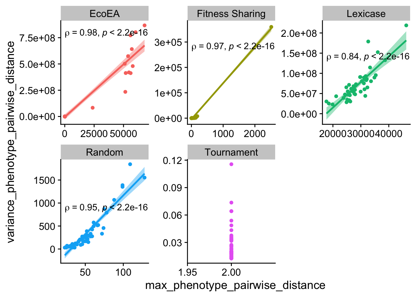

Max and variance of pairwise distances behave similarly.

And let’s check that it doesn’t look radically different early on in the run:

ggplot(
    data %>% filter(gen==5000),
    aes(
        y=mean_phenotype_pairwise_distance,
        x=variance_phenotype_pairwise_distance,
        color=selection_name,
        fill=selection_name
    )
  ) +
  geom_point() +
  scale_x_continuous(
        breaks = breaks_extended(4)
  ) + 
  facet_wrap(
      ~selection_name, scales="free"
  ) + 
  stat_smooth(
    method="lm"
  ) + 
  stat_cor(
    method="spearman", cor.coef.name = "rho", color="black"
  ) +
  theme(legend.position = "none")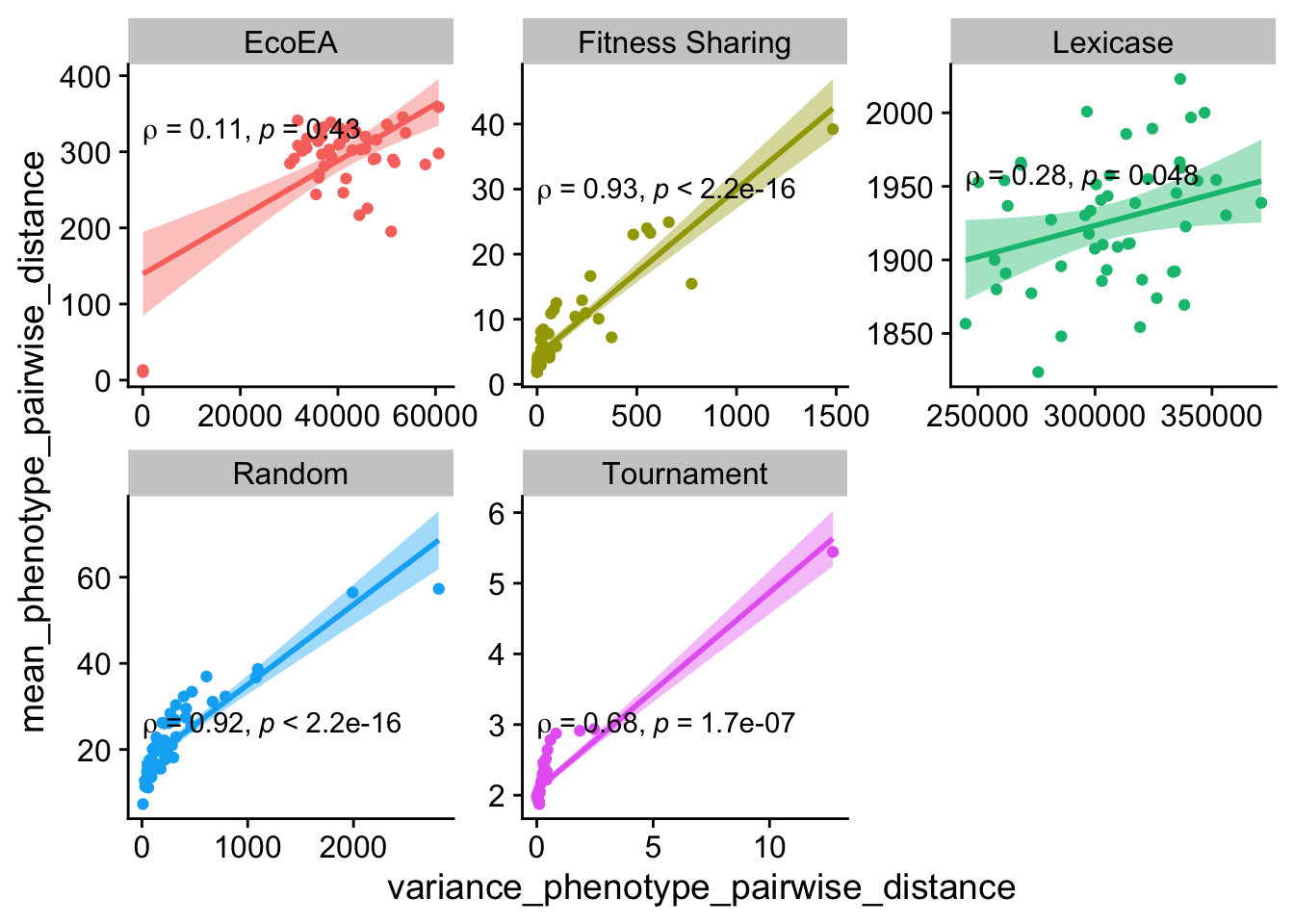

The correlation between these two metrics is substantially weaker for Eco-Ea and lexicase selection at the early time point.

ggplot(
    data %>% filter(gen==5000),
    aes(
        y=mean_phenotype_pairwise_distance,
        x=max_phenotype_pairwise_distance,
        color=selection_name,
        fill=selection_name
    )
  ) +
  geom_point() +
  scale_x_continuous(
        breaks = breaks_extended(4)
  ) + 
  facet_wrap(
      ~selection_name, scales="free"
  ) + 
  stat_smooth(
    method="lm"
  ) + 
  stat_cor(
    method="spearman", cor.coef.name = "rho", color="black"
  ) +
  theme(legend.position = "none")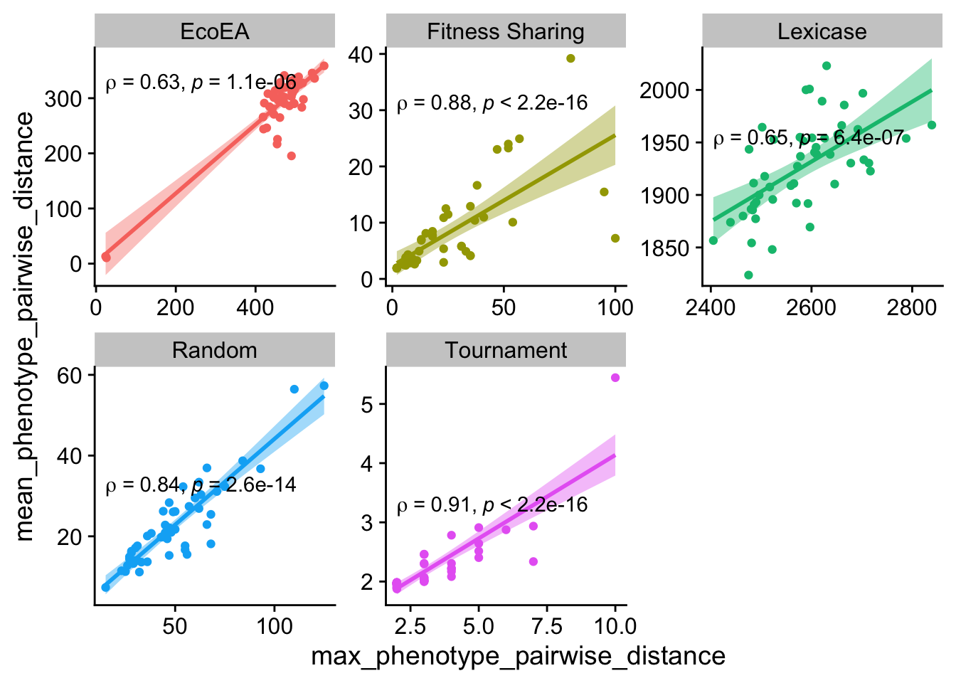

This relationship is also weaker, although not as much weaker.

ggplot(
    data %>% filter(gen==5000),
    aes(
        y=variance_phenotype_pairwise_distance,
        x=max_phenotype_pairwise_distance,
        color=selection_name,
        fill=selection_name
    )
  ) +
  geom_point() +
  scale_x_continuous(
        breaks = breaks_extended(4)
  ) + 
  facet_wrap(
      ~selection_name, scales="free"
  ) + 
  stat_smooth(
    method="lm"
  ) + 
  stat_cor(
    method="spearman", cor.coef.name = "rho", color="black"
  ) +
  theme(legend.position = "none")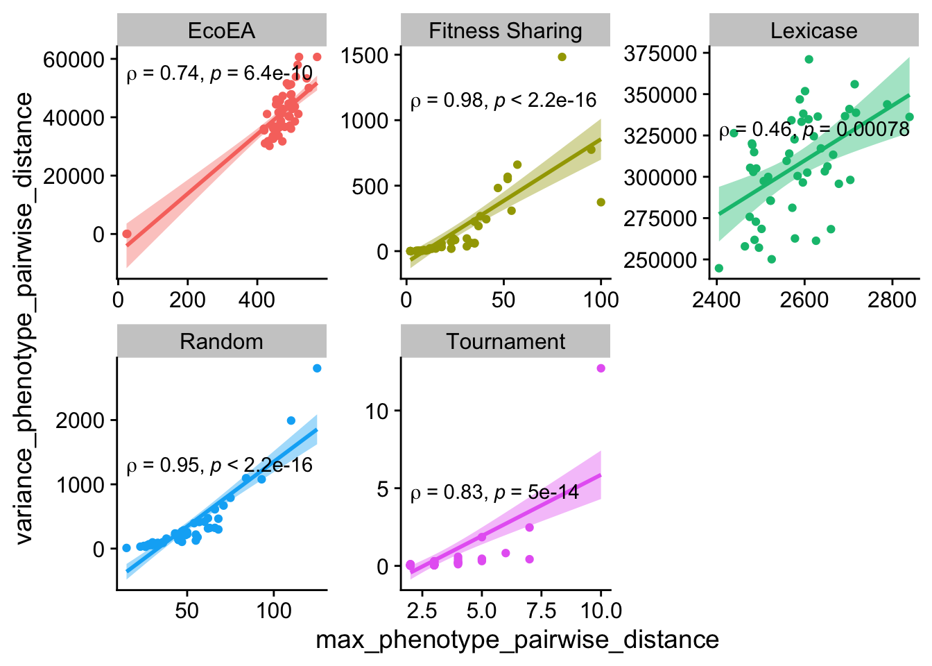

Similarly, the correlation between max and variance of pariwise distances is weakend, but still robust. So the relationship between mean and variance of pairwise distances is the only one that is really weaker at the earlier time points. Understanding exactly what drives these discrepancies is a promising angle for future work, as it may shed further light on the dynamics occurring in the run. It is particularly interesting that EcoEA and Lexicase selection are the scenarios where they diverge.

Similarly, the evolutionary distinctiveness metrics look largely similar to each other, but let’s spot check that too.

ggplot(
    data %>% filter(gen==500000),
    aes(
        y=mean_phenotype_evolutionary_distinctiveness,
        x=variance_phenotype_evolutionary_distinctiveness,
        color=selection_name,
        fill=selection_name
    )
  ) +
  geom_point() +
  scale_x_continuous(
        breaks = breaks_extended(4)
  ) + 
  facet_wrap(
      ~selection_name, scales="free"
  ) + 
  stat_smooth(
    method="lm"
  ) + 
  stat_cor(
    method="spearman", cor.coef.name = "rho", color="black"
  ) +
  theme(legend.position = "none")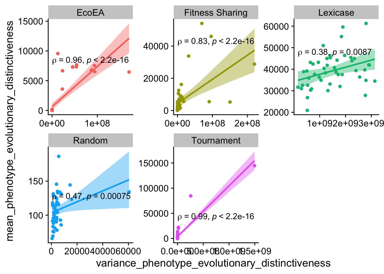

These aren’t the strongest correlations; different information is definitely being captured by each metric. However, they still correlate to a fair extent.

ggplot(
    data %>% filter(gen==500000),
    aes(
        y=mean_phenotype_evolutionary_distinctiveness,
        x=max_phenotype_evolutionary_distinctiveness,
        color=selection_name,
        fill=selection_name
    )
  ) +
  geom_point() +
  scale_x_continuous(
        breaks = breaks_extended(4)
  ) + 
  facet_wrap(
      ~selection_name, scales="free"
  ) + 
  stat_smooth(
    method="lm"
  ) + 
  stat_cor(
    method="spearman", cor.coef.name = "rho", color="black"
  ) +
  theme(legend.position = "none")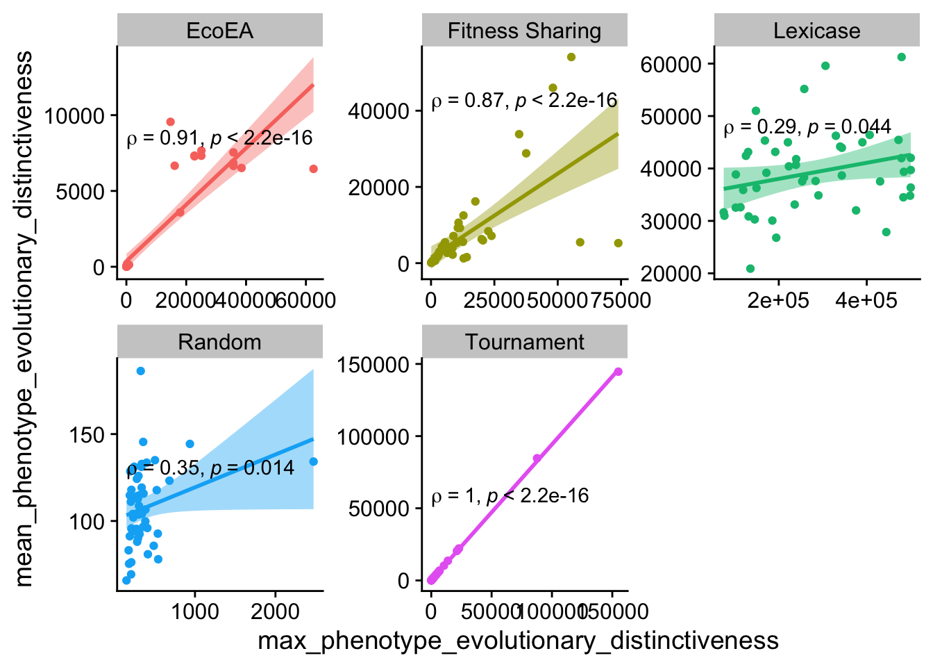

Again, for the most part there is a fairly high degree of correlation here.

ggplot(
    data %>% filter(gen==500000),
    aes(
        y=mean_phenotype_evolutionary_distinctiveness,
        x=min_phenotype_evolutionary_distinctiveness,
        color=selection_name,
        fill=selection_name
    )
  ) +
  geom_point() +
  scale_x_continuous(
        breaks = breaks_extended(4)
  ) + 
  facet_wrap(
      ~selection_name, scales="free"
  ) + 
  stat_smooth(
    method="lm"
  ) + 
  stat_cor(
    method="spearman", cor.coef.name = "rho", color="black"
  ) +
  theme(legend.position = "none")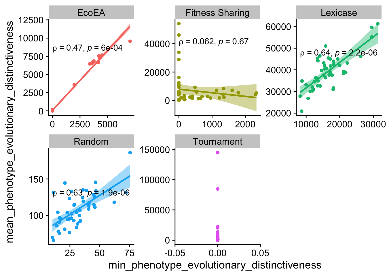

And here too, although it’s getting kind of weak for lexicase.

And let’s check out an earlier time point

ggplot(
    data %>% filter(gen==5000),
    aes(
        y=mean_phenotype_evolutionary_distinctiveness,
        x=variance_phenotype_evolutionary_distinctiveness,
        color=selection_name,
        fill=selection_name
    )
  ) +
  geom_point() +
  scale_x_continuous(
        breaks = breaks_extended(4)
  ) + 
  facet_wrap(
      ~selection_name, scales="free"
  ) + 
  stat_smooth(
    method="lm"
  ) + 
  stat_cor(
    method="spearman", cor.coef.name = "rho", color="black"
  ) +
  theme(legend.position = "none")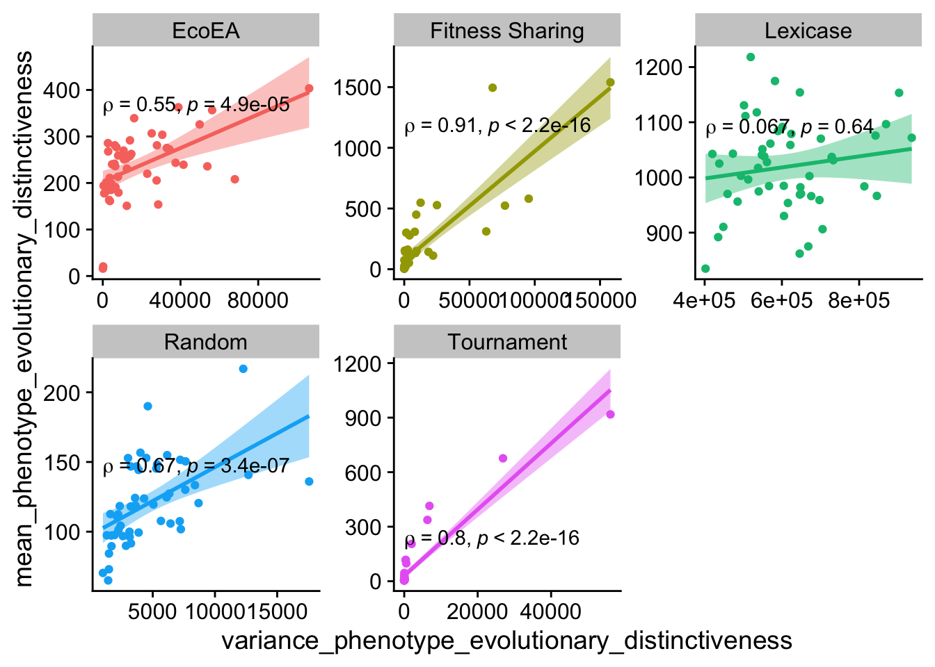

The relationship between min and mean evolutionary distinctiveness holds up at the earlier time point for everything except fitness sharing.

ggplot(
    data %>% filter(gen==5000),
    aes(
        y=mean_phenotype_evolutionary_distinctiveness,
        x=max_phenotype_evolutionary_distinctiveness,
        color=selection_name,
        fill=selection_name
    )
  ) +
  geom_point() +
  scale_x_continuous(
        breaks = breaks_extended(4)
  ) + 
  facet_wrap(
      ~selection_name, scales="free"
  ) + 
  stat_smooth(
    method="lm"
  ) + 
  stat_cor(
    method="spearman", cor.coef.name = "rho", color="black"
  ) +
  theme(legend.position = "none")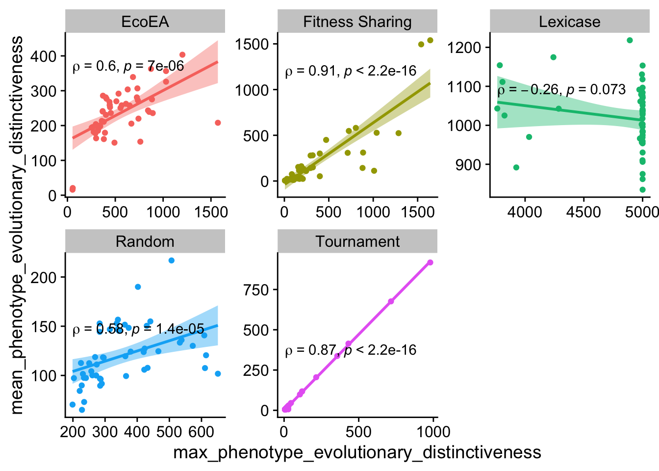

And here, for everything except lexicase

ggplot(
    data %>% filter(gen==5000),
    aes(
        y=mean_phenotype_evolutionary_distinctiveness,
        x=min_phenotype_evolutionary_distinctiveness,
        color=selection_name,
        fill=selection_name
    )
  ) +
  geom_point() +
  scale_x_continuous(
        breaks = breaks_extended(4)
  ) + 
  facet_wrap(
      ~selection_name, scales="free"
  ) + 
  stat_smooth(
    method="lm"
  ) + 
  stat_cor(
    method="spearman", cor.coef.name = "rho", color="black"
  ) +
  theme(legend.position = "none")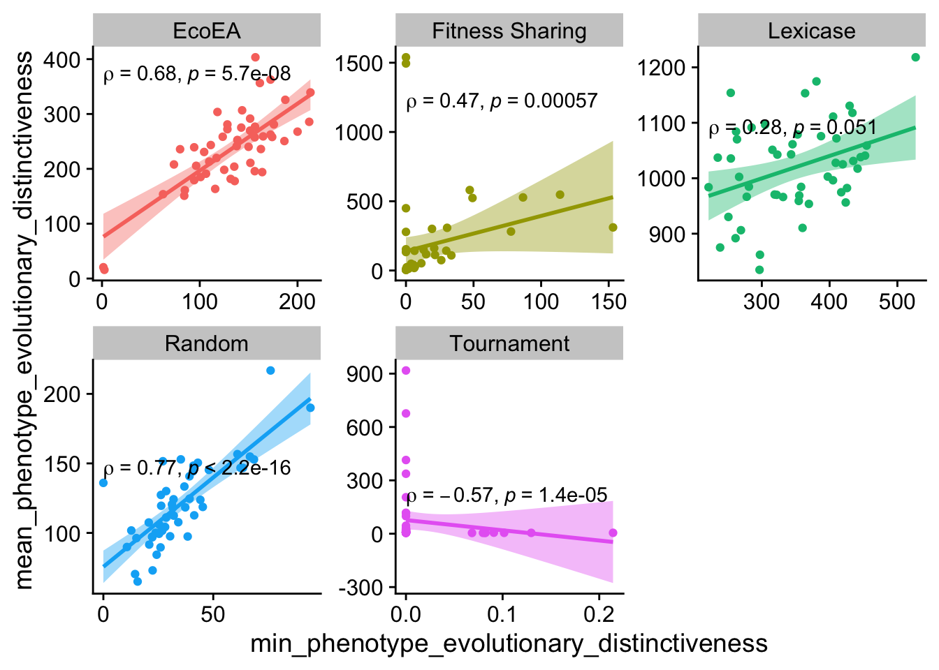

These are relatively weak for the most part.

Looks like the evolutionary distinctiveness statistics capture more different information from each other than the pairwise distance statistics (in general the correlations are weaker, and there are more deviations from the pattern of positive correlations). However, in a lot of cases they still correlate. There is definitely more exploration to be done on what differences in these metrics imply, but for simplicity we’ll stick to one pairwise distance metric and one evolutionary distinctiveness metric.

Since it’s hard to get a gestalt impression from the scatterplots, let’s take a look at the correlation matrices for each selection scheme. Note that these are at the final time point, which clearly misses some dynamics that occurr earlier.

2.3.1.1 Random

final_data %>% 
  filter(selection_name=="Random") %>%
  transmute(MinPD=min_phenotype_pairwise_distance, 
            MeanPD=mean_phenotype_pairwise_distance, 
            MaxPD=max_phenotype_pairwise_distance, 
            VarPD=variance_phenotype_pairwise_distance, 
            MinED = min_phenotype_evolutionary_distinctiveness,
            MeanED= mean_phenotype_evolutionary_distinctiveness,
            MaxED=max_phenotype_evolutionary_distinctiveness,
            VarED=variance_phenotype_evolutionary_distinctiveness,
            PD=phenotype_current_phylogenetic_diversity,  # See Faith 1992
            MRCA=phen_mrca_depth,  # Phylogenetic depth of most recent common ancestor
            N=phen_num_taxa     # Number of taxonomically-distinct phenotypes
  ) %>%
  cor_mat() %>% 
  pull_lower_triangle() %>% 
  cor_plot()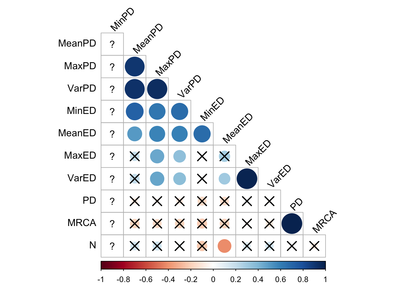

In random selection, all the pairwise distance metrics correlate with each other, and also more weakly with some of the evolutionary distinctiveness metrics, but not max and variance (although they correlate strongly with each other). It is somewhat surprising that the depth of the most recent common ancestor and Faith’s Phylogenetic Diveristy metric have so little correlation with the others.

2.3.1.2 Tournament

final_data %>% 
  filter(selection_name=="Tournament") %>%
  transmute(MinPD=min_phenotype_pairwise_distance, 
            MeanPD=mean_phenotype_pairwise_distance, 
            MaxPD=max_phenotype_pairwise_distance, 
            VarPD=variance_phenotype_pairwise_distance, 
            MinED = min_phenotype_evolutionary_distinctiveness,
            MeanED= mean_phenotype_evolutionary_distinctiveness,
            MaxED=max_phenotype_evolutionary_distinctiveness,
            VarED=variance_phenotype_evolutionary_distinctiveness,
            PD=phenotype_current_phylogenetic_diversity,  # See Faith 1992
            MRCA=phen_mrca_depth,  # Phylogenetic depth of most recent common ancestor
            N=phen_num_taxa     # Number of taxonomically-distinct phenotypes
  ) %>%
  cor_mat() %>% 
  pull_lower_triangle() %>% 
  cor_plot()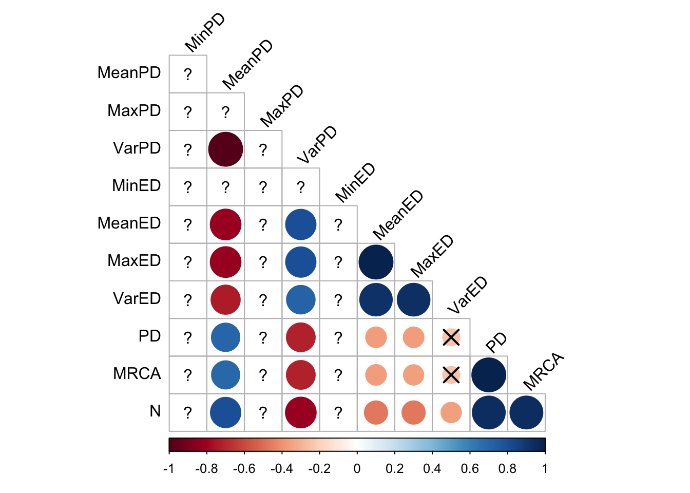

Here, all the evolutionary distinctiveness metrics coreelate strongly with each other, but the pairiwse distance metrics less so (although this is likely an artifact of the extremely low phylogenetic diversity in tournament selection)

2.3.1.3 Fitness Sharing

final_data %>% 
  filter(selection_name=="Fitness Sharing") %>%
  transmute(MinPD=min_phenotype_pairwise_distance, 
            MeanPD=mean_phenotype_pairwise_distance, 
            MaxPD=max_phenotype_pairwise_distance, 
            VarPD=variance_phenotype_pairwise_distance, 
            MinED = min_phenotype_evolutionary_distinctiveness,
            MeanED= mean_phenotype_evolutionary_distinctiveness,
            MaxED=max_phenotype_evolutionary_distinctiveness,
            VarED=variance_phenotype_evolutionary_distinctiveness,
            PD=phenotype_current_phylogenetic_diversity,  # See Faith 1992
            MRCA=phen_mrca_depth,  # Phylogenetic depth of most recent common ancestor
            N=phen_num_taxa     # Number of taxonomically-distinct phenotypes
  ) %>%
  cor_mat() %>% 
  pull_lower_triangle() %>% 
  cor_plot()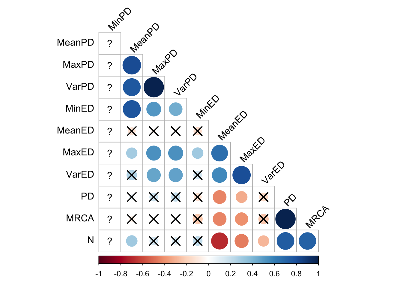

Here, the pairwise distance metrics correlate with each other and the evolutionary distinctivenes metrics correlated with each other. There are some correlations between pairwise distance and evolutionary distinctiveness metrics, but they’re weaker.

2.3.1.4 Lexicase selection

final_data %>% 
  filter(selection_name=="Lexicase") %>%
  transmute(MinPD=min_phenotype_pairwise_distance, 
            MeanPD=mean_phenotype_pairwise_distance, 
            MaxPD=max_phenotype_pairwise_distance, 
            VarPD=variance_phenotype_pairwise_distance, 
            MinED = min_phenotype_evolutionary_distinctiveness,
            MeanED= mean_phenotype_evolutionary_distinctiveness,
            MaxED=max_phenotype_evolutionary_distinctiveness,
            VarED=variance_phenotype_evolutionary_distinctiveness,
            PD=phenotype_current_phylogenetic_diversity,  # See Faith 1992
            MRCA=phen_mrca_depth,  # Phylogenetic depth of most recent common ancestor
            N=phen_num_taxa     # Number of taxonomically-distinct phenotypes
  ) %>%
  cor_mat() %>% 
  pull_lower_triangle() %>% 
  cor_plot()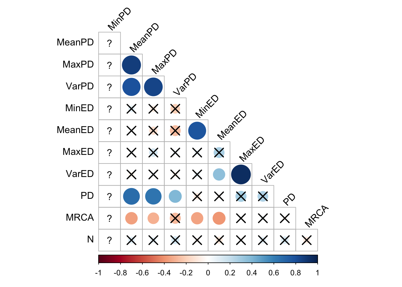

Again, the pairwise distance metrics correlate with each other but not wth the volutionary distinctivness metrics. The evolutionary distinctiveness metrics sort of correlate with each other.

2.3.1.5 Eco-EA

final_data %>% 
  filter(selection_name=="EcoEA") %>%
  transmute(MinPD=min_phenotype_pairwise_distance, 
            MeanPD=mean_phenotype_pairwise_distance, 
            MaxPD=max_phenotype_pairwise_distance, 
            VarPD=variance_phenotype_pairwise_distance, 
            MinED = min_phenotype_evolutionary_distinctiveness,
            MeanED= mean_phenotype_evolutionary_distinctiveness,
            MaxED=max_phenotype_evolutionary_distinctiveness,
            VarED=variance_phenotype_evolutionary_distinctiveness,
            PD=phenotype_current_phylogenetic_diversity,  # See Faith 1992
            MRCA=phen_mrca_depth,  # Phylogenetic depth of most recent common ancestor
            N=phen_num_taxa     # Number of taxonomically-distinct phenotypes
  ) %>%
  cor_mat() %>% 
  pull_lower_triangle() %>% 
  cor_plot()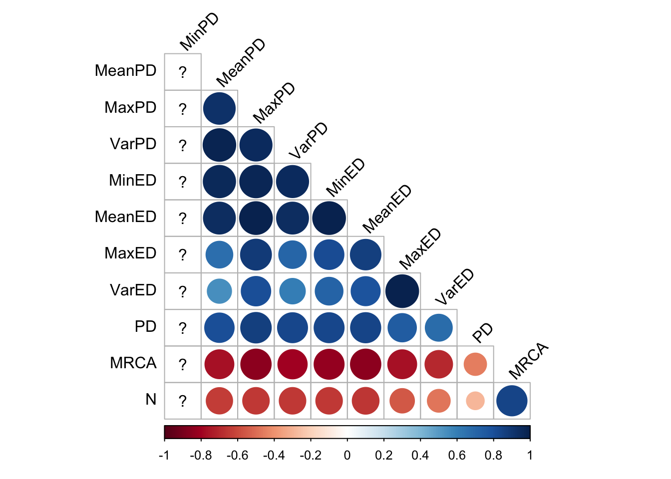

In Eco-EA, there is an impressively strong positive correlation among all the phylodiversity metrics. Understanding what causes Eco-EA to deviate from lexicase selection (and to a lesser extent fitness sharing) in this way would be worthy of further research.

2.3.2 Over time

2.3.2.1 Mean pairwise distance

First we plot mean pairwise distance over time. We log the y axis because there is such variation in mean pairwise distance across selection schemes, and the x-axis for the same reason as before.

ggplot(
    data,
    aes(
      x=gen,
      y=mean_phenotype_pairwise_distance,
      color=selection_name,
      fill=selection_name
    )
  ) +
  stat_summary(geom="line", fun=mean) +
  stat_summary(
    geom="ribbon",
    fun.data="mean_cl_boot",
    fun.args=list(conf.int=0.95),
    alpha=0.2,
    linetype=0
  ) +
  scale_y_log10(
    name="Mean pairwise distance"
  ) +
  scale_x_log10(
    name="Generation"
  ) +
  scale_color_discrete("Selection") +
  scale_fill_discrete("Selection")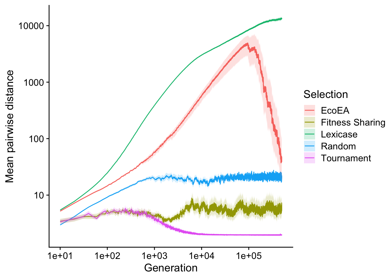

Lexicase selection maintains a monotonic increase in phylogenetic diversity over the course of the entire experiment. It likely never experiences a full coalescence event (where the most-recent common ancestor changes). Eco-EA nearly keeps pace with lexicase selection until towards the end, when its phylogenetic diversity crashes. This is likely the result of selective sweeps that begin to occur as the population discovers high fitness solutions. Fitness sharing shows a slight dip at the same time that its fitness plateaus (likely also the result of a selective sweep), but phylogenetic diversity recovers afterwards, making for a relatively constant level. over time. Tournament selection, on the other hand, maintains the same (low) level of phylogenetic diversity as fitness sharing, up until the point that fitness plateaus, at which point tournament selection’s phylodiversity drops to nearly 0. Interestingly, lexicase selection and Eco-EA both maintain more phylodiversity than random selection, whereas fitness sharing and tournament selection maintain less.

2.3.2.2 Mean evolutionary distinctiveness

For comparison, we make the same plot with mean evolutionary distinctiveness.

ggplot(
    data,
    aes(
      x=gen,
      y=mean_phenotype_evolutionary_distinctiveness,
      color=selection_name,
      fill=selection_name
    )
  ) +
  stat_summary(geom="line", fun=mean) +
  stat_summary(
    geom="ribbon",
    fun.data="mean_cl_boot",
    fun.args=list(conf.int=0.95),
    alpha=0.2,
    linetype=0
  ) +
  scale_y_log10(
    name="Mean evolutionary distinctiveness"
  ) +
  scale_x_log10(
    name="Generation"
  ) +
  scale_color_discrete("Selection") +
  scale_fill_discrete("Selection")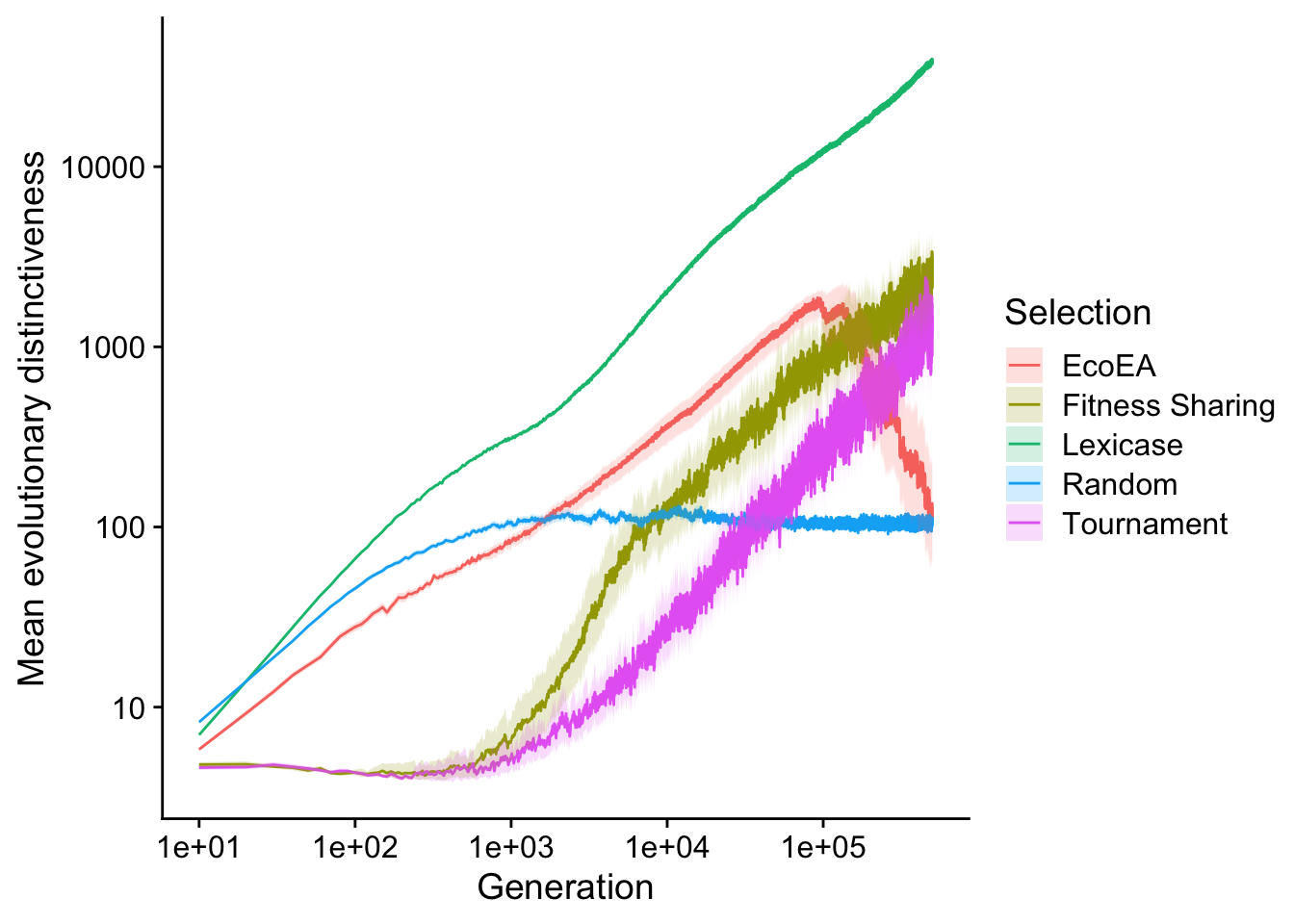

Interestingly, Fitness Sharing and tournament selection both start increasing in evolutionary distinctiveness only after their fitnesses have plateaued. This seems likely to be due to some sort of pathological behavior of mean evolutionary distinctiveness on small trees, but more investigation would be necessary to figure out exactly what’s going on. Trends in other selection schemes are largely similar.

2.3.3 Final

Next, we perform a more in-depth analysis of phylodiversity distributions at the final time point.

2.3.3.1 Mean pairwise distance

First, we test which selection schemes end up with significantly different final distributions of mean pairwise distance.

# Pairwise wilcoxon teset to determine which conditions are significantly different from each other
stat.test <- final_data %>%
  wilcox_test(mean_phenotype_pairwise_distance ~ selection_name) %>%
  adjust_pvalue(method = "bonferroni") %>%
  add_significance() %>%
  add_xy_position(x="selection_name",step.increase=1)
stat.test$label <- mapply(p_label,stat.test$p.adj)

# Output stats
stat.test %>%
  kbl() %>%
  kable_styling(
    bootstrap_options = c(
      "striped",
      "hover",
      "condensed",
      "responsive"
    )
  ) %>%
  scroll_box(width="600px")

.y.	group1	group2	n1	n2	statistic	p	p.adj	p.adj.signif	y.position	groups	xmin	xmax	label
mean_phenotype_pairwise_distance	EcoEA	Fitness Sharing	50	50	1824.0	7.70e-05	7.70e-04	***	49488.81	EcoEA , Fitness Sharing	1	2	p = 0.00077
mean_phenotype_pairwise_distance	EcoEA	Lexicase	50	47	227.0	0.00e+00	0.00e+00	****	76981.49	EcoEA , Lexicase	1	3	p < 1e-04
mean_phenotype_pairwise_distance	EcoEA	Random	50	50	690.0	1.15e-04	1.15e-03	**	104474.18	EcoEA , Random	1	4	p = 0.00115
mean_phenotype_pairwise_distance	EcoEA	Tournament	50	50	2500.0	0.00e+00	0.00e+00	****	131966.86	EcoEA , Tournament	1	5	p < 1e-04
mean_phenotype_pairwise_distance	Fitness Sharing	Lexicase	50	47	0.0	0.00e+00	0.00e+00	****	159459.54	Fitness Sharing, Lexicase	2	3	p < 1e-04
mean_phenotype_pairwise_distance	Fitness Sharing	Random	50	50	536.0	9.00e-07	8.70e-06	****	186952.22	Fitness Sharing, Random	2	4	p < 1e-04
mean_phenotype_pairwise_distance	Fitness Sharing	Tournament	50	50	2232.5	0.00e+00	0.00e+00	****	214444.90	Fitness Sharing, Tournament	2	5	p < 1e-04
mean_phenotype_pairwise_distance	Lexicase	Random	47	50	2350.0	0.00e+00	0.00e+00	****	241937.58	Lexicase, Random	3	4	p < 1e-04
mean_phenotype_pairwise_distance	Lexicase	Tournament	47	50	2350.0	0.00e+00	0.00e+00	****	269430.26	Lexicase , Tournament	3	5	p < 1e-04
mean_phenotype_pairwise_distance	Random	Tournament	50	50	2500.0	0.00e+00	0.00e+00	****	296922.94	Random , Tournament	4	5	p < 1e-04

Looks like they are all significantly different from each other.

# Raincloud plot of final mean pairwise distance
final_phylogeny_fig <- ggplot(
    final_data,
    aes(
      x=selection_name,
      y=mean_phenotype_pairwise_distance,
      fill=selection_name
    )
  ) +
  geom_flat_violin(
    position = position_nudge(x = .2, y = 0),
    alpha = .8,
    scale="width"
  ) +
  geom_point(
    mapping=aes(color=selection_name),
    position = position_jitter(width = .15),
    size = .5,
    alpha = 0.8
  ) +
  geom_boxplot(
    width = .1,
    outlier.shape = NA,
    alpha = 0.5
  ) +
  scale_y_log10(
    name="Mean pairwise distance"
  ) +
  scale_x_discrete(
    name="Selection"
  ) +
  scale_fill_discrete(
    name="Selection"
  ) +
  scale_color_discrete(
    name="Selection"
  ) + 
  theme(legend.position = "none")
final_phylogeny_fig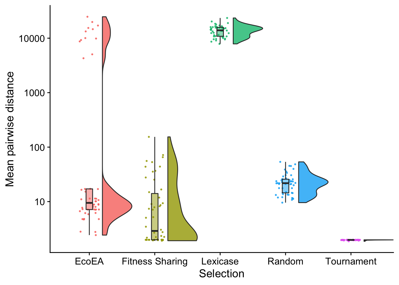

This shows something interesting! Final phylogenetic diversity in Eco-EA is heavily bimodal. In later analysis, we will see that the runs with high phylogenetic diversity are the ones with lower fitness, suggesting that they have no yet experienced a selective sweep resulting from the discovery of a high-fitness solution.

2.3.3.2 Mean evolutionary distinctiveness

Tests for significant differences:

# Pairwise wilcoxon teset to determine which conditions are significantly different from each other
stat.test <- final_data %>%
  wilcox_test(mean_phenotype_evolutionary_distinctiveness ~ selection_name) %>%
  adjust_pvalue(method = "bonferroni") %>%
  add_significance() %>%
  add_xy_position(x="selection_name",step.increase=1)
stat.test$label <- mapply(p_label,stat.test$p.adj)

# Output stats

stat.test %>%
  kbl() %>%
  kable_styling(
    bootstrap_options = c(
      "striped",
      "hover",
      "condensed",
      "responsive"
    )
  ) %>%
  scroll_box(width="100%")

.y.	group1	group2	n1	n2	statistic	p	p.adj	p.adj.signif	y.position	groups	xmin	xmax	label
mean_phenotype_evolutionary_distinctiveness	EcoEA	Fitness Sharing	50	50	469	1.00e-07	7.00e-07	****	289111.7	EcoEA , Fitness Sharing	1	2	p < 1e-04
mean_phenotype_evolutionary_distinctiveness	EcoEA	Lexicase	50	47	0	0.00e+00	0.00e+00	****	449625.8	EcoEA , Lexicase	1	3	p < 1e-04
mean_phenotype_evolutionary_distinctiveness	EcoEA	Random	50	50	711	2.05e-04	2.05e-03	**	610140.0	EcoEA , Random	1	4	p = 0.00205
mean_phenotype_evolutionary_distinctiveness	EcoEA	Tournament	50	50	569	2.70e-06	2.72e-05	****	770654.1	EcoEA , Tournament	1	5	p < 1e-04
mean_phenotype_evolutionary_distinctiveness	Fitness Sharing	Lexicase	50	47	100	0.00e+00	0.00e+00	****	931168.2	Fitness Sharing, Lexicase	2	3	p < 1e-04
mean_phenotype_evolutionary_distinctiveness	Fitness Sharing	Random	50	50	2428	0.00e+00	0.00e+00	****	1091682.4	Fitness Sharing, Random	2	4	p < 1e-04
mean_phenotype_evolutionary_distinctiveness	Fitness Sharing	Tournament	50	50	1614	1.20e-02	1.20e-01	ns	1252196.5	Fitness Sharing, Tournament	2	5	p = 0.12
mean_phenotype_evolutionary_distinctiveness	Lexicase	Random	47	50	2350	0.00e+00	0.00e+00	****	1412710.6	Lexicase, Random	3	4	p < 1e-04
mean_phenotype_evolutionary_distinctiveness	Lexicase	Tournament	47	50	2255	0.00e+00	0.00e+00	****	1573224.7	Lexicase , Tournament	3	5	p < 1e-04
mean_phenotype_evolutionary_distinctiveness	Random	Tournament	50	50	173	0.00e+00	0.00e+00	****	1733738.9	Random , Tournament	4	5	p < 1e-04

Looks like everything except fitness sharing and tournament are significantly different from each other.

# Raincloud plot of final mean evolutionary distinctiveness
ggplot(
    final_data,
    aes(
      x=selection_name,
      y=mean_phenotype_evolutionary_distinctiveness,
      fill=selection_name
    )
  ) +
  geom_flat_violin(
    position = position_nudge(x = .2, y = 0),
    alpha = .8,
    scale="width"
  ) +
  geom_point(
    mapping=aes(color=selection_name),
    position = position_jitter(width = .15),
    size = .5,
    alpha = 0.8
  ) +
  geom_boxplot(
    width = .1,
    outlier.shape = NA,
    alpha = 0.5
  ) +
  scale_y_log10(
    name="Mean evolutionary distinctiveness"
  ) +
  scale_x_discrete(
    name="Selection"
  ) +
  scale_fill_discrete(
    name="Selection"
  ) +
  scale_color_discrete(
    name="Selection"
  ) + 
  theme(legend.position = "none")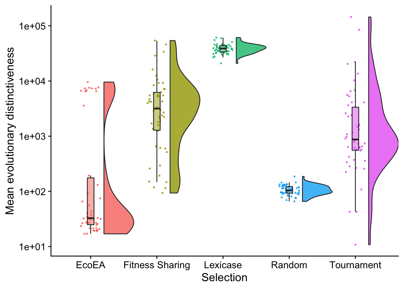

Again, this looks fairly similar to MPD, except that fitness sharing and tournament are higher.

2.4 Phenotypic diversity

Now we analyze phenotypic (i.e. population-level) diversity. Here, we’re defining phenotypes to only include the sites that are actively contributing to fitness. So the phenotype of [1,4,2,6,5,4,3,6,7] would be [0,0,0,6,5,4,3,0,0]. Note that phylogenetic trees are also built using this conception of phenotypes.

2.4.1 Relationship between different types of phenotypic diversity

First, we should assess the extent to which different metrics of phenotypic diversity are capturing different information.

ggplot(
    data %>% filter(gen==500000),
    aes(
        y=phen_diversity,
        x=phen_num_taxa,
        color=selection_name,
        fill=selection_name
    )
  ) +
  geom_point() +
    scale_y_continuous(
        name="Phenotypic shannon diversity"
  ) +
  scale_x_continuous(
        name="Phenotypic richness",
        breaks = breaks_extended(4)
  ) + 
  facet_wrap(
      ~selection_name, scales="free"
  ) + 
  stat_smooth(
    method="lm"
  ) + 
  stat_cor(
    method="spearman", cor.coef.name = "rho", color="black"
  ) +
  theme(legend.position = "none")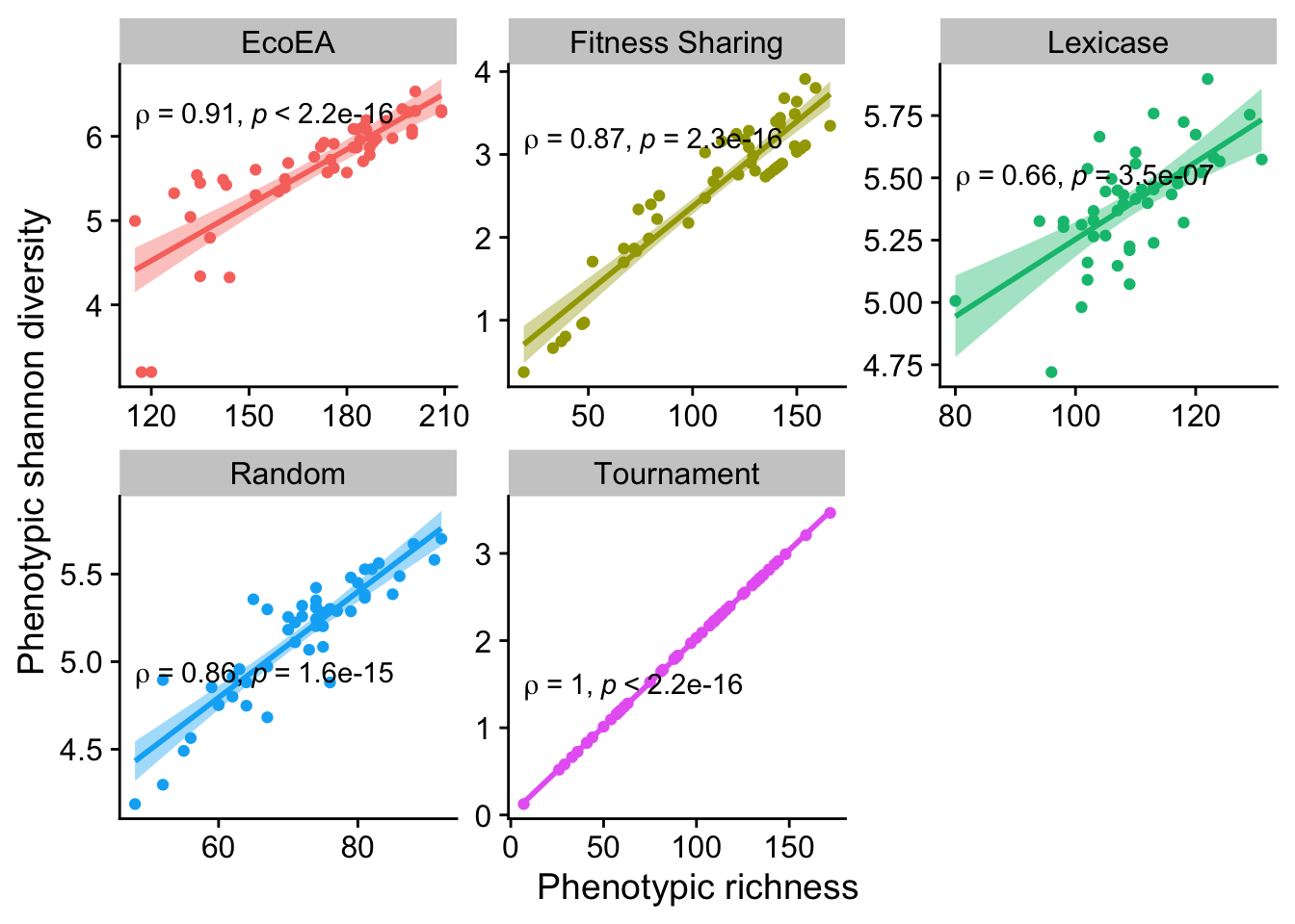

Looks like at the final time point they are pretty much always closely correlated, although this correlation is weaker for lexicase selection than for other selection schemes.

2.4.2 Over time

Now we examine the behavior of each phenotypic diversity metric over time.

2.4.2.1 Richness

ggplot(
    data,
    aes(
      x=gen,
      y=phen_num_taxa,
      color=selection_name,
      fill=selection_name
    )
  ) +
  stat_summary(geom="line", fun=mean) +
  stat_summary(
    geom="ribbon",
    fun.data="mean_cl_boot",
    fun.args=list(conf.int=0.95),
    alpha=0.2,
    linetype=0
  ) +
  scale_y_continuous(
    name="Phenotypic richness"
  ) +
  scale_x_log10(
    name="Generation"
  ) +
  scale_color_discrete("Selection") + 
  scale_fill_discrete("Selection")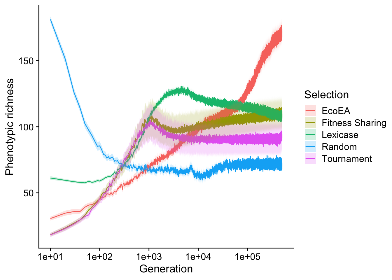

In contrast to the phylodiversity results, phenotypic richness in all selection schemes (even tournament selection) ultimately exceeds that of random selection. Eco-EA monotonically increases while lexicase selection reaches a maximum around the same time it reaches its fitness plateau. The only real similarity to the phylodiversity results is the behavior tournament selection and fitness sharing relative to each other.

2.4.2.2 Shannon diversity

We also looked at phenotypic shannon diversity:

ggplot(
    data,
    aes(
      x=gen,
      y=phen_diversity,
      color=selection_name,
      fill=selection_name
    )
  ) +
  stat_summary(geom="line", fun=mean) +
  stat_summary(
    geom="ribbon",
    fun.data="mean_cl_boot",
    fun.args=list(conf.int=0.95),
    alpha=0.2,
    linetype=0
  ) +
  scale_y_continuous(
    name="Phenotypic Shannon entropy"
  ) +
  scale_x_log10(
    name="Generation"
  ) +
  scale_color_discrete("Selection") + 
  scale_fill_discrete("Selection")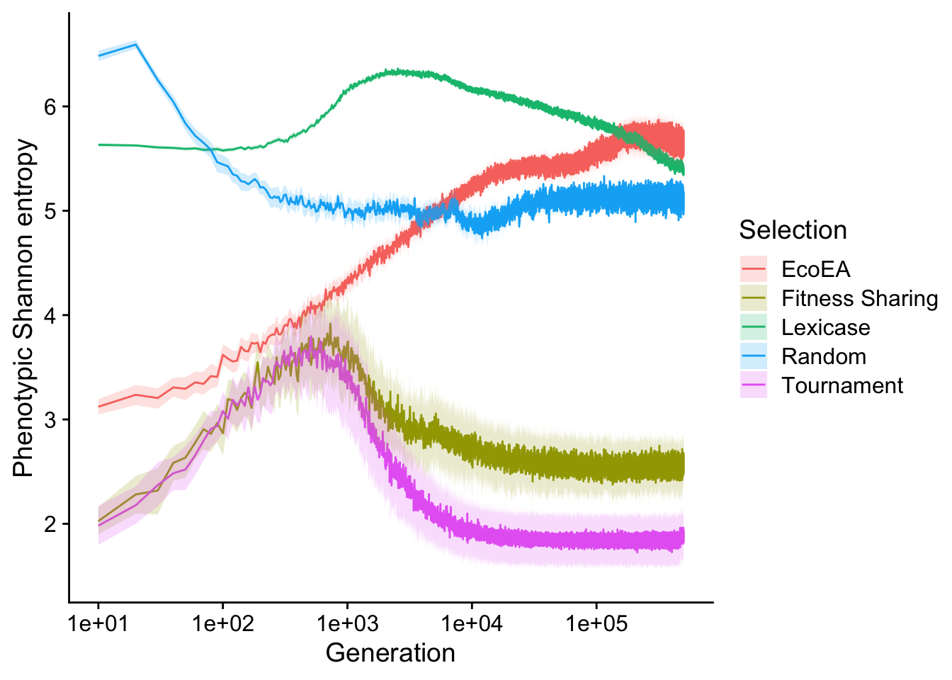

This is more different from the richness results than we might have expected based on the correlation at the final time point. There is a much more pronounced drop off in Shannon entropy for tournament and fitness sharing than in richness. This difference is probably driven by the fact that, after plateauing, these selection schemes are likely both at mutation-selection balance. Thus, there are very many single-mutant phenotypes with only one copy in the population. These do not contribute much to Shannon entropy or phylogenetic diversity, but it does show up in richness.

We also see that, after plataeuing, lexicase selection does actually start to decrease in Shannon entropy, but slowly. Similarly, in Eco-EA, the increase in Shannon entropy towards the end is much more modest than the increase in richness.

2.4.3 Final

Now we assess the final phenotypic diversity

2.4.3.1 Richness

Hypothesis-testing differences between groups:

# Determine which conditions are significantly diferrent from each other
stat.test <- final_data %>%
  wilcox_test(phen_num_taxa ~ selection_name) %>%
  adjust_pvalue(method = "bonferroni") %>%
  add_significance() %>%
  add_xy_position(x="selection_name",step.increase=1)
stat.test$label <- mapply(p_label,stat.test$p.adj)

stat.test %>%
  kbl() %>%
  kable_styling(
    bootstrap_options = c(
      "striped",
      "hover",
      "condensed",
      "responsive"
    )
  ) %>%
  scroll_box(width="600px")

.y.	group1	group2	n1	n2	statistic	p	p.adj	p.adj.signif	y.position	groups	xmin	xmax	label
phen_num_taxa	EcoEA	Fitness Sharing	50	50	2249.0	0.00e+00	0.0e+00	****	326	EcoEA , Fitness Sharing	1	2	p < 1e-04
phen_num_taxa	EcoEA	Lexicase	50	47	2319.0	0.00e+00	0.0e+00	****	456	EcoEA , Lexicase	1	3	p < 1e-04
phen_num_taxa	EcoEA	Random	50	50	2500.0	0.00e+00	0.0e+00	****	586	EcoEA , Random	1	4	p < 1e-04
phen_num_taxa	EcoEA	Tournament	50	50	2378.5	0.00e+00	0.0e+00	****	716	EcoEA , Tournament	1	5	p < 1e-04
phen_num_taxa	Fitness Sharing	Lexicase	50	47	1428.0	6.80e-02	6.8e-01	ns	846	Fitness Sharing, Lexicase	2	3	p = 0.68
phen_num_taxa	Fitness Sharing	Random	50	50	1973.0	6.00e-07	6.3e-06	****	976	Fitness Sharing, Random	2	4	p < 1e-04
phen_num_taxa	Fitness Sharing	Tournament	50	50	1585.0	2.10e-02	2.1e-01	ns	1106	Fitness Sharing, Tournament	2	5	p = 0.21
phen_num_taxa	Lexicase	Random	47	50	2339.5	0.00e+00	0.0e+00	****	1236	Lexicase, Random	3	4	p < 1e-04
phen_num_taxa	Lexicase	Tournament	47	50	1359.0	1.85e-01	1.0e+00	ns	1366	Lexicase , Tournament	3	5	p = 1
phen_num_taxa	Random	Tournament	50	50	797.0	2.00e-03	2.0e-02		1496	Random , Tournament	4	5	p = 0.02

Raincloud plot:

# Raincloud plot of final phenotypic diversity
final_phenotypic_fig <- ggplot(
    final_data,
    aes(
      x=selection_name,
      y=phen_num_taxa,
      fill=selection_name
    )
  ) +
  geom_flat_violin(
    position = position_nudge(x = .2, y = 0),
    alpha = .8,
    scale="width"
  ) +
  geom_point(
    mapping=aes(color=selection_name),
    position = position_jitter(width = .15),
    size = .5,
    alpha = 0.8
  ) +
  geom_boxplot(
    width = .1,
    outlier.shape = NA,
    alpha = 0.5
  ) +
  scale_y_continuous(
    name="Phenotypic Richness"
  ) +
  scale_x_discrete(
    name="Selection"
  ) +
  scale_fill_discrete(
    name="Selection"
  ) +
  scale_color_discrete(
    name="Selection"
  ) +
  theme(legend.position = "none")
final_phenotypic_fig

Nothing particularly suprising here, but we should note that, based on the over time plot, this would look a lot different if we had selected a different time point.

2.4.3.2 Shannon diversity

# Determine which conditions are significantly diferrent from each other
stat.test <- final_data %>%
  wilcox_test(phen_diversity~ selection_name) %>%
  adjust_pvalue(method = "bonferroni") %>%
  add_significance() %>%
  add_xy_position(x="selection_name",step.increase=1)
stat.test$label <- mapply(p_label,stat.test$p.adj)

stat.test %>%
  kbl() %>%
  kable_styling(
    bootstrap_options = c(
      "striped",
      "hover",
      "condensed",
      "responsive"
    )
  ) %>%
  scroll_box(width="600px")

.y.	group1	group2	n1	n2	statistic	p	p.adj	p.adj.signif	y.position	groups	xmin	xmax	label
phen_diversity	EcoEA	Fitness Sharing	50	50	2478.0	0.00e+00	0.00e+00	****	9.602	EcoEA , Fitness Sharing	1	2	p < 1e-04
phen_diversity	EcoEA	Lexicase	50	47	1772.0	1.66e-05	1.66e-04	***	13.012	EcoEA , Lexicase	1	3	p = 0.000166
phen_diversity	EcoEA	Random	50	50	2089.5	0.00e+00	1.00e-07	****	16.422	EcoEA , Random	1	4	p < 1e-04
phen_diversity	EcoEA	Tournament	50	50	2496.0	0.00e+00	0.00e+00	****	19.832	EcoEA , Tournament	1	5	p < 1e-04
phen_diversity	Fitness Sharing	Lexicase	50	47	0.0	0.00e+00	0.00e+00	****	23.242	Fitness Sharing, Lexicase	2	3	p < 1e-04
phen_diversity	Fitness Sharing	Random	50	50	0.0	0.00e+00	0.00e+00	****	26.652	Fitness Sharing, Random	2	4	p < 1e-04
phen_diversity	Fitness Sharing	Tournament	50	50	1856.0	2.99e-05	2.99e-04	***	30.062	Fitness Sharing, Tournament	2	5	p = 0.000299
phen_diversity	Lexicase	Random	47	50	1714.0	1.01e-04	1.01e-03	**	33.472	Lexicase, Random	3	4	p = 0.00101
phen_diversity	Lexicase	Tournament	47	50	2350.0	0.00e+00	0.00e+00	****	36.882	Lexicase , Tournament	3	5	p < 1e-04
phen_diversity	Random	Tournament	50	50	2500.0	0.00e+00	0.00e+00	****	40.292	Random , Tournament	4	5	p < 1e-04

Interestingly, the final shannon diversity values of different selection schemes are much more distinguishable from each other than the final richness values.

# Raincloud plot of final phenotypic diversity
ggplot(
    final_data,
    aes(
      x=selection_name,
      y=phen_num_taxa,
      fill=selection_name
    )
  ) +
  geom_flat_violin(
    position = position_nudge(x = .2, y = 0),
    alpha = .8,
    scale="width"
  ) +
  geom_point(
    mapping=aes(color=selection_name),
    position = position_jitter(width = .15),
    size = .5,
    alpha = 0.8
  ) +
  geom_boxplot(
    width = .1,
    outlier.shape = NA,
    alpha = 0.5
  ) +
  scale_y_continuous(
    name="Phenotypic Shannon Diversity"
  ) +
  scale_x_discrete(
    name="Selection"
  ) +
  scale_fill_discrete(
    name="Selection"
  ) +
  scale_color_discrete(
    name="Selection"
  ) +
  theme(legend.position = "none")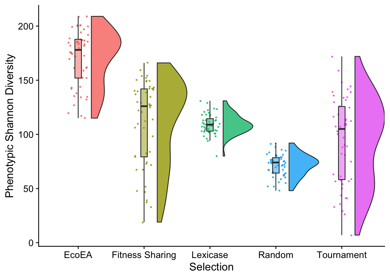

Again, we know from the time series plots that these relative relationships varied a lot over time. Eco-EA is only higher than lexicase selection at the very end.

2.5 Relationship between phenotypic and phylogenetic diversity

Now, we can finally begin to address the main questions. Do phenotypic diversity and phylogenetic diversity capture different information?

2.5.1 Phenotypic richness vs. mean pairwise distance

ggplot(
    data %>% filter(gen==500000),
    aes(
        y=phen_num_taxa,
        x=mean_phenotype_pairwise_distance,
        color=selection_name,
        fill=selection_name
    )
  ) +
  geom_point() +
    scale_y_continuous(
        name="Phenotypic richness"
  ) +
  scale_x_continuous(
        name="Mean pairwise distance",
        breaks = breaks_extended(4)
  ) + 
  facet_wrap(
      ~selection_name, scales="free"
  ) + 
  stat_smooth(
    method="lm"
  ) + 
  stat_cor(
    method="spearman", cor.coef.name = "rho", color="black"
  ) +
  theme(legend.position = "none")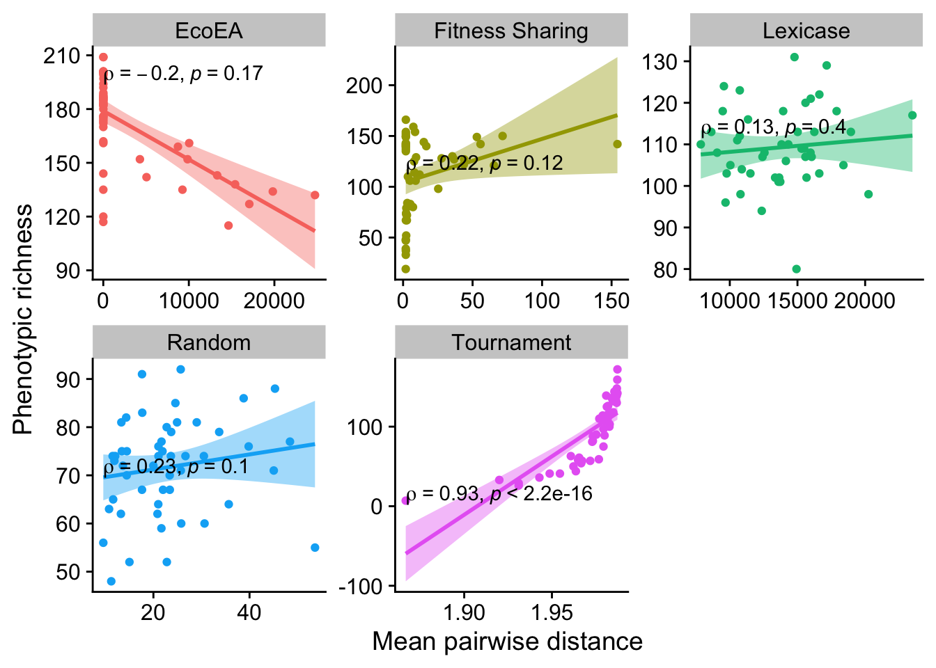

The linear models for some of these are questionable, but the Spearman correlation coefficient should be fine because it does not require linearity. Only tournament selection is significantly different from 0. Eco-EA is even negative (although non-significant), which is probably driven by the fact that there are really two groups of runs in Eco-EA: those that have found a good solution and had their diversity crash, and those that haven’t yet.

Lets take a look at how each of those groups behave (we’ll show fitness as color, just to better understand what’s happening):

ggplot(
    data %>% filter(gen==500000, selection_name == "EcoEA"),
    aes(
        y=phen_num_taxa,
        x=mean_phenotype_pairwise_distance,
        color = elite_trait_avg
    )
  ) +
  geom_point() +
    scale_y_continuous(
        name="Phenotypic richness"
  ) +
  scale_x_continuous(
        name="Mean pairwise distance",
        breaks = breaks_extended(4)
  ) + 
  facet_wrap(
      ~mean_phenotype_pairwise_distance > 100, scales="free"
  ) + 
  stat_smooth(
    method="lm"
  ) + 
  stat_cor(
    method="spearman", cor.coef.name = "rho", color="black"
  ) +
  scale_color_continuous(type="viridis")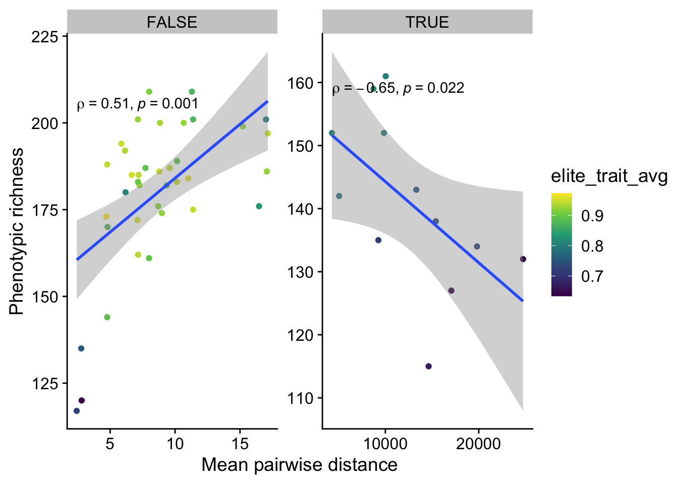

2.5.2 Phenotypic richness vs. mean evolutionary distinctiveness

ggplot(
    data %>% filter(gen==500000),
    aes(
        y=phen_num_taxa,
        x=mean_phenotype_evolutionary_distinctiveness,
        color=selection_name,
        fill=selection_name
    )
  ) +
  geom_point() +
    scale_y_continuous(
        name="Phenotypic richness"
  ) +
  scale_x_continuous(
        name="Mean evolutionary distinctiveness",
        breaks = breaks_extended(4)
  ) + 
  facet_wrap(
      ~selection_name, scales="free"
  ) + 
  stat_smooth(
    method="lm"
  ) + 
  stat_cor(
    method="spearman", cor.coef.name = "rho", color="black"
  ) +
  theme(legend.position = "none")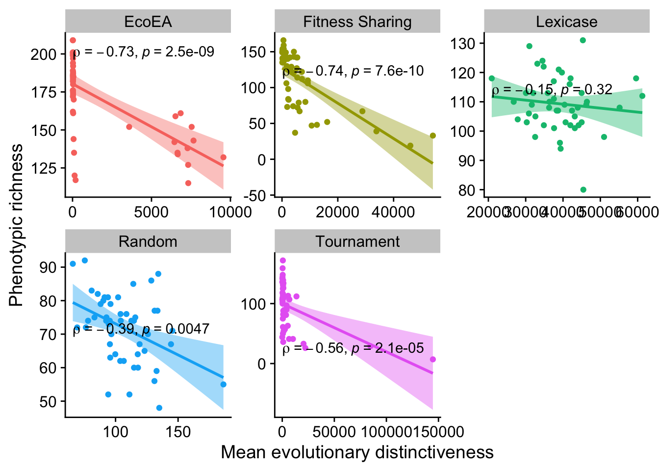

These are mostly significant, but negative. That’s interesting and worthy of further exploration (but it’s a little beyond the scope of this analysis).

2.5.3 Phenotypic shannon diversity vs. mean pairwise distance

ggplot(
    data %>% filter(gen==500000),
    aes(
        y=phen_diversity,
        x=mean_phenotype_pairwise_distance,
        color=selection_name,
        fill=selection_name
    )
  ) +
  geom_point() +
    scale_y_continuous(
        name="Phenotypic shannon diversity"
  ) +
  scale_x_continuous(
        name="Mean pairwise distance",
        breaks = breaks_extended(4)
  ) + 
  facet_wrap(
      ~selection_name, scales="free"
  ) + 
  stat_smooth(
    method="lm"
  ) + 
  stat_cor(
    method="spearman", cor.coef.name = "rho", color="black"
  ) +
  theme(legend.position = "none")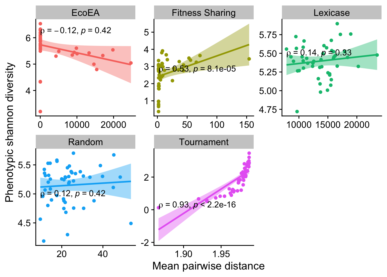

Again, these are mostly not significant (although fitness sharing notably now is).

2.5.4 Phenotypic shannon diversity vs. mean evolutionary distinctiveness

ggplot(
    data %>% filter(gen==500000),
    aes(
        y=phen_diversity,
        x=mean_phenotype_evolutionary_distinctiveness,
        color=selection_name,
        fill=selection_name
    )
  ) +
  geom_point() +
    scale_y_continuous(
        name="Phenotypic shannon diversity"
  ) +
  scale_x_continuous(
        name="Mean evolutionary distinctiveness",
        breaks = breaks_extended(4)
  ) + 
  facet_wrap(
      ~selection_name, scales="free"
  ) + 
  stat_smooth(
    method="lm"
  ) + 
  stat_cor(
    method="spearman", cor.coef.name = "rho", color="black"
  ) +
  theme(legend.position = "none")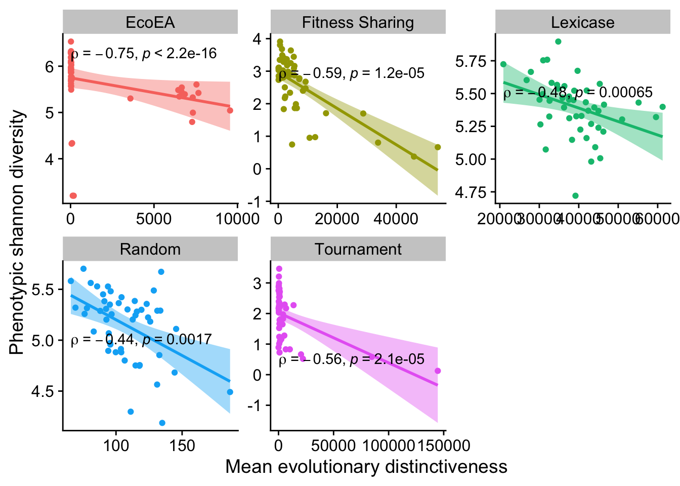

Again, all significant but negative. From this we can conclude that there is substantially more overlap between the information captured by phenotypic diversity and mean evolutionary disinctiveness than between phenotypic diversity metrics and mean pairwise distance. However, thus information has wildly different implications in the two contexts. Moreover, the long term trends are still very different. Thus, we still feel confident in saying that these metrics are meaningfully different. More investigation here may be worthwhile in the future.

Overall, based on these end of time analyses and qualitative comparison of the temporal graphs, we conclude that phenotypic and phylogenetic diversity are meaningfully different from each other in the context of evolutionary computation. In retrospect, this finding may seem obvious. However a lot of people tend to assume that these two classes of diversity are closely related.

2.6 Relationship between diversity and success

At last, we can finally assess whether diversity leads to actually solving problems! We start out by looking at correlations between diversity success across a few different time points, although we ultimately conclude that this approach is not particularly informative.

2.6.1 Very early in run

2.6.1.1 Mean pairwise distance

ggplot(
    data %>% filter(gen==25000),
    aes(
        y=elite_trait_avg,
        x=mean_phenotype_pairwise_distance,
        color=selection_name,
        fill=selection_name
    )
  ) +
  geom_point() +
    scale_y_continuous(
        name="Average trait performance"
  ) +
  scale_x_continuous(
        name="Mean pairwise distance"
  ) + 
  facet_wrap(
      ~selection_name, scales="free"
  ) + 
  stat_smooth(
    method="lm"
  ) + 
  stat_cor(
    method="spearman", cor.coef.name = "rho", color="black"
  ) +
  theme(legend.position = "none")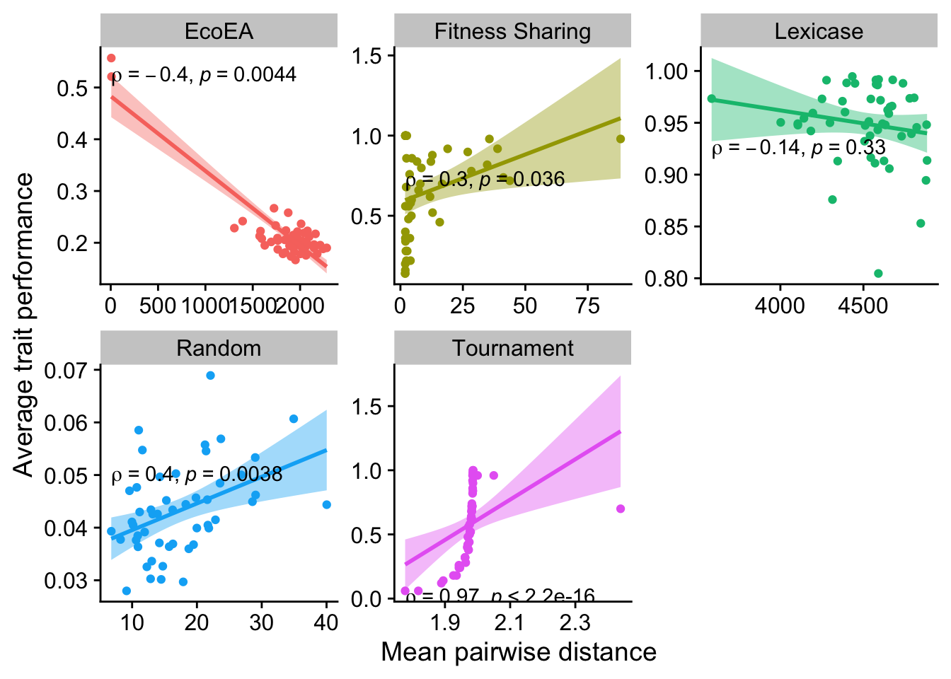

2.6.1.2 Mean evolutionary distinctiveness

ggplot(
    data %>% filter(gen==25000),
    aes(
        y=elite_trait_avg,
        x=mean_phenotype_evolutionary_distinctiveness,
        color=selection_name,
        fill=selection_name
    )
  ) +
  geom_point() +
    scale_y_continuous(
        name="Average trait performance"
  ) +
  scale_x_continuous(
        name="Mean evolutionary distinctiveness"
  ) + 
  facet_wrap(
      ~selection_name, scales="free"
  ) + 
  stat_smooth(
    method="lm"
  ) + 
  stat_cor(
    method="spearman", cor.coef.name = "rho", color="black"
  ) +
  theme(legend.position = "none")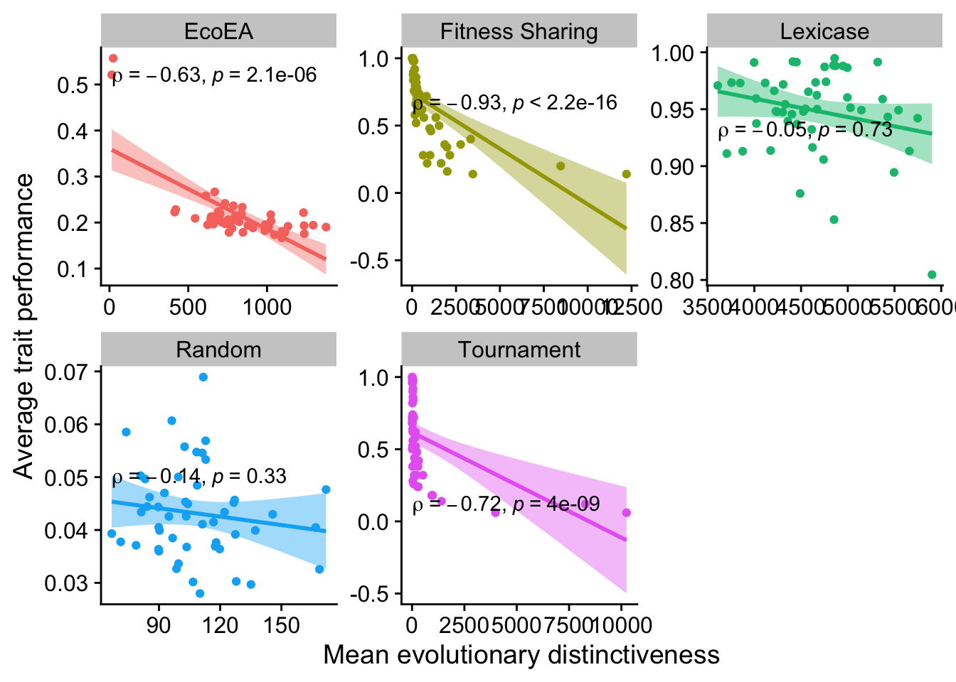

2.6.1.3 Richness

ggplot(
    data %>% filter(gen==25000),
    aes(
        y=elite_trait_avg,
        x=phen_num_taxa,
        color=selection_name,
        fill=selection_name
    )
  ) +
  geom_point() +
    scale_y_continuous(
        name="Average trait performance"
  ) +
  scale_x_continuous(
        name="Phenotypic richness"
  ) + 
  facet_wrap(
      ~selection_name, scales="free"
  ) + 
  stat_smooth(
    method="lm"
  ) + 
  stat_cor(
    method="spearman", cor.coef.name = "rho", color="black"
  ) +
  theme(legend.position = "none")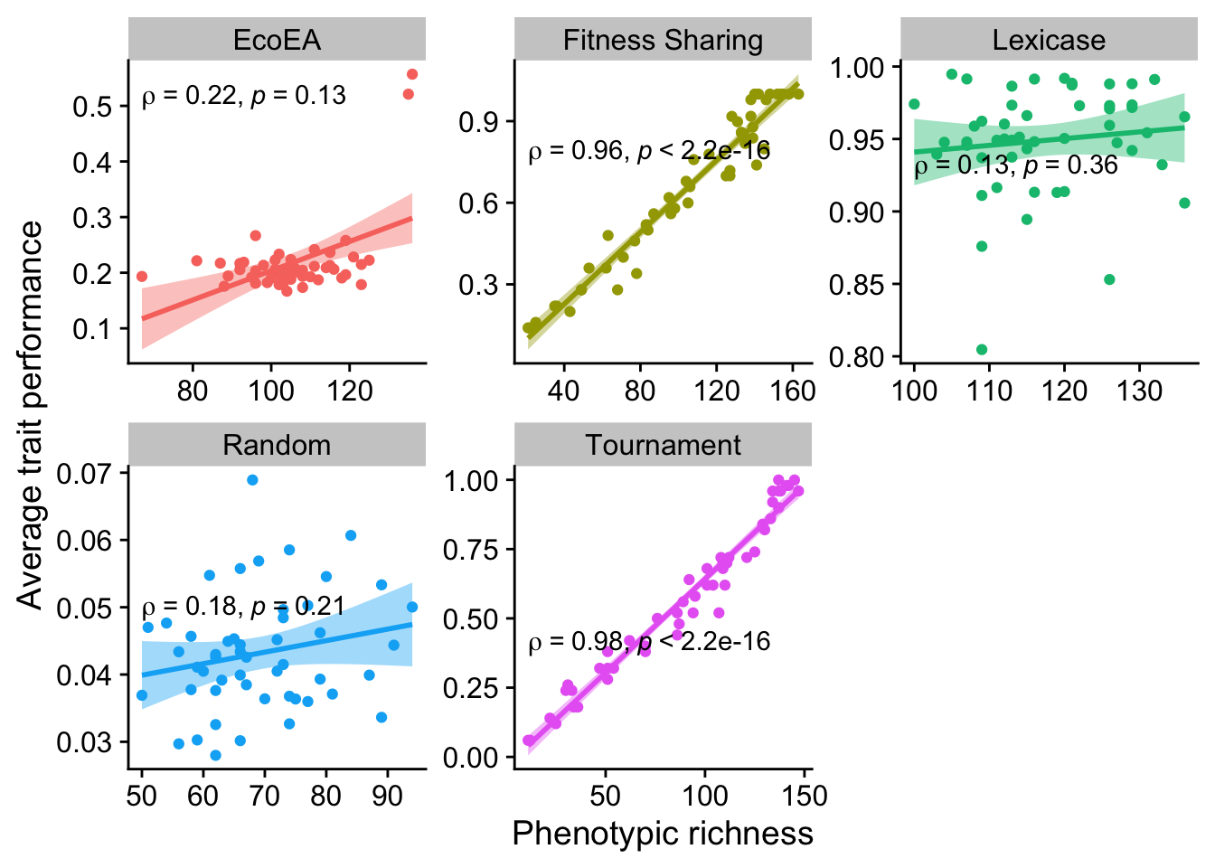

2.6.1.4 Shannon diversity

ggplot(
    data %>% filter(gen==25000),
    aes(
        y=elite_trait_avg,
        x=phen_diversity,
        color=selection_name,
        fill=selection_name
    )
  ) +
  geom_point() +
    scale_y_continuous(
        name="Average trait performance"
  ) +
  scale_x_continuous(
        name="Phenotypic Shannon diversity"
  ) + 
  facet_wrap(
      ~selection_name, scales="free"
  ) + 
  stat_smooth(
    method="lm"
  ) + 
  stat_cor(
    method="spearman", cor.coef.name = "rho", color="black"
  ) +
  theme(legend.position = "none")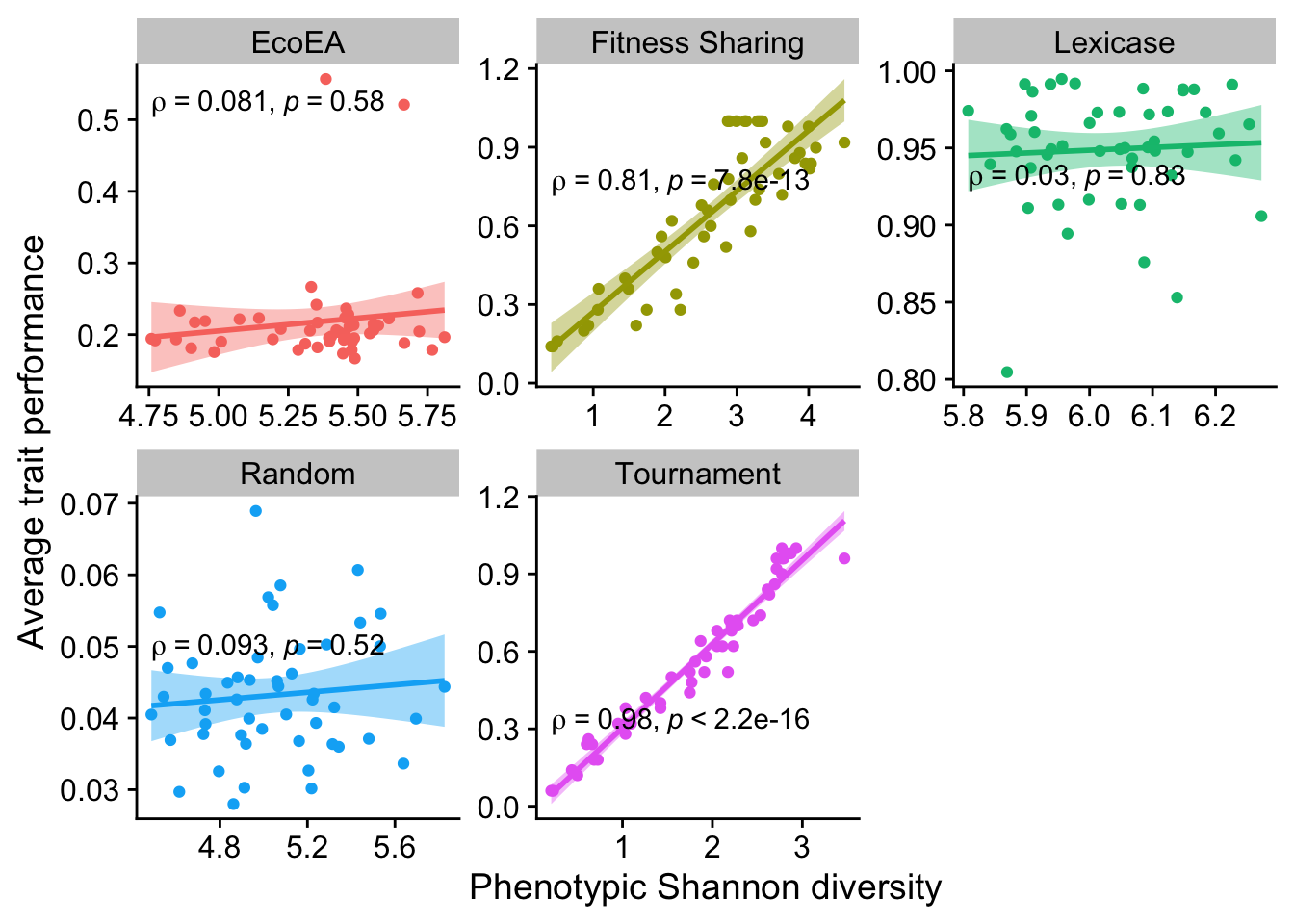

2.6.2 Middle of run

2.6.2.1 Mean pairwise distance

ggplot(
    data %>% filter(gen==50000),
    aes(
        y=elite_trait_avg,
        x=mean_phenotype_pairwise_distance,
        color=selection_name,
        fill=selection_name
    )
  ) +
  geom_point() +
    scale_y_continuous(
        name="Average trait performance"
  ) +
  scale_x_continuous(
        name="Mean pairwise distance"
  ) + 
  facet_wrap(
      ~selection_name, scales="free"
  ) + 
  stat_smooth(
    method="lm"
  ) + 
  stat_cor(
    method="spearman", cor.coef.name = "rho", color="black"
  ) +
  theme(legend.position = "none")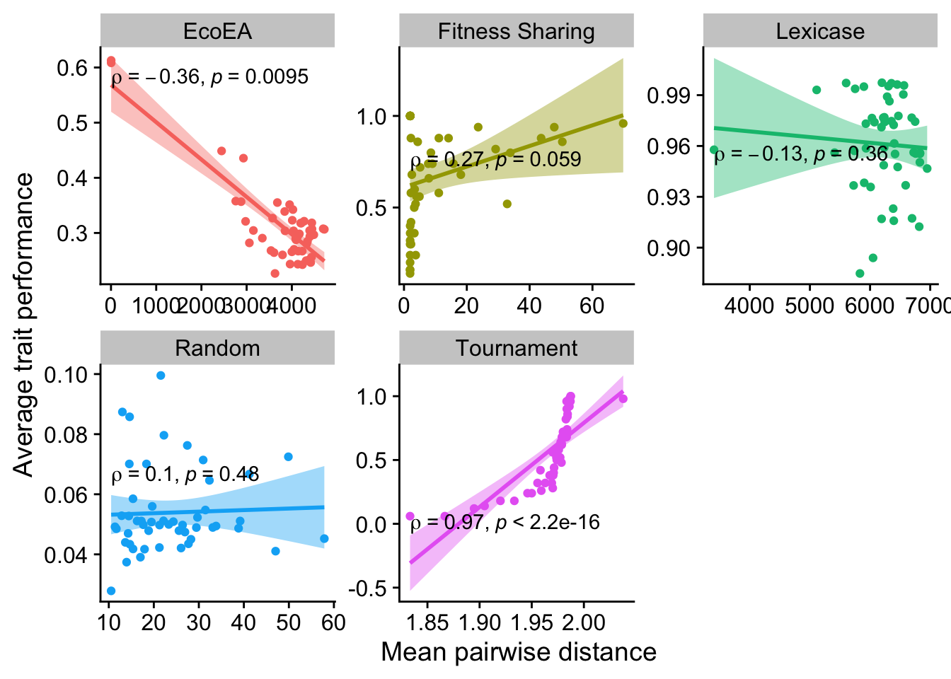

2.6.2.2 Mean evolutionary distinctiveness

ggplot(
    data %>% filter(gen==50000),
    aes(
        y=elite_trait_avg,
        x=mean_phenotype_evolutionary_distinctiveness,
        color=selection_name,
        fill=selection_name
    )
  ) +
  geom_point() +
    scale_y_continuous(
        name="Average trait performance"
  ) +
  scale_x_continuous(
        name="Mean evolutionary distinctiveness"
  ) + 
  facet_wrap(
      ~selection_name, scales="free"
  ) + 
  stat_smooth(
    method="lm"
  ) + 
  stat_cor(
    method="spearman", cor.coef.name = "rho", color="black"
  ) +
  theme(legend.position = "none")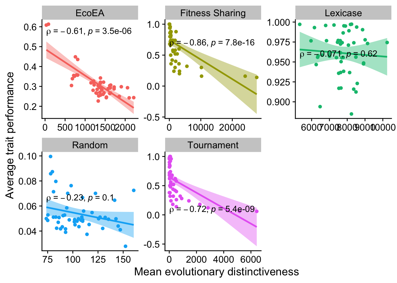

2.6.2.3 Richness

ggplot(
    data %>% filter(gen==50000),
    aes(
        y=elite_trait_avg,
        x=phen_num_taxa,
        color=selection_name,
        fill=selection_name
    )
  ) +
  geom_point() +
    scale_y_continuous(
        name="Average trait performance"
  ) +
  scale_x_continuous(
        name="Phenotypic richness"
  ) + 
  facet_wrap(
      ~selection_name, scales="free"
  ) + 
  stat_smooth(
    method="lm"
  ) + 
  stat_cor(
    method="spearman", cor.coef.name = "rho", color="black"
  ) +
  theme(legend.position = "none")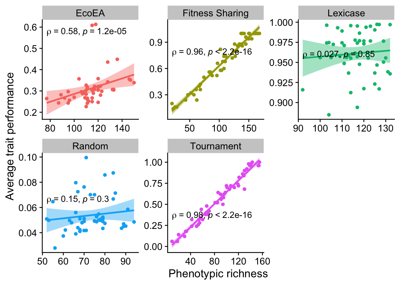

2.6.2.4 Shannon diversity

ggplot(
    data %>% filter(gen==50000),
    aes(
        y=elite_trait_avg,
        x=phen_diversity,
        color=selection_name,
        fill=selection_name
    )
  ) +
  geom_point() +
    scale_y_continuous(
        name="Average trait performance"
  ) +
  scale_x_continuous(
        name="Phenotypic Shannon diversity"
  ) + 
  facet_wrap(
      ~selection_name, scales="free"
  ) + 
  stat_smooth(
    method="lm"
  ) + 
  stat_cor(
    method="spearman", cor.coef.name = "rho", color="black"
  ) +
  theme(legend.position = "none")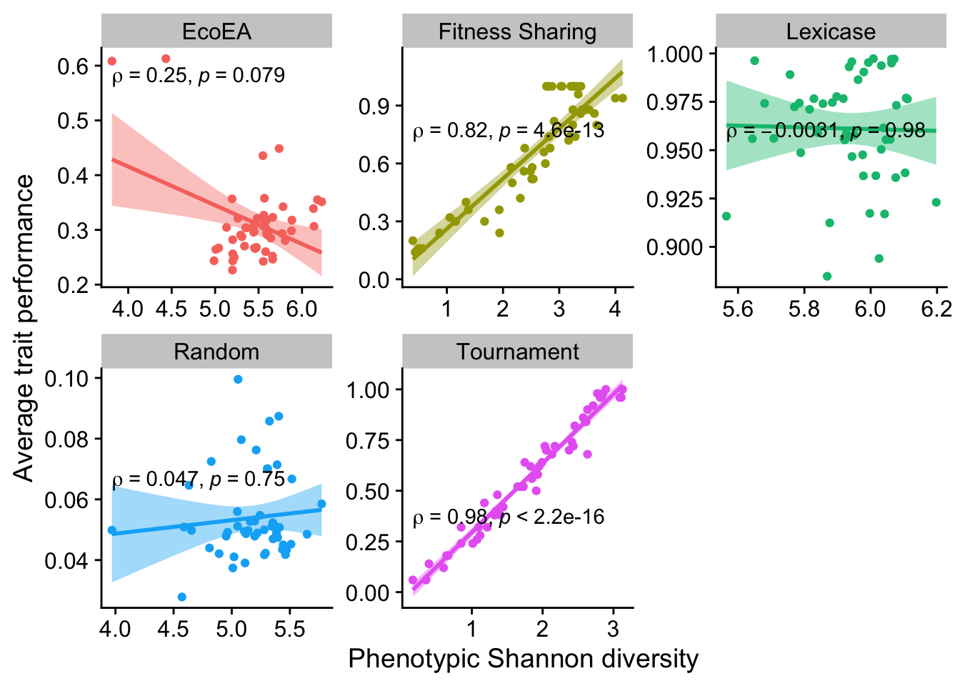

2.6.3 End of run

2.6.3.1 Mean pairwise distance

ggplot(
    final_data,
    aes(
        y=elite_trait_avg,
        x=mean_phenotype_pairwise_distance,
        color=selection_name,
        fill=selection_name
    )
  ) +
  geom_point() +
    scale_y_continuous(
        name="Average trait performance"
  ) +
  scale_x_continuous(
        name="Mean pairwise distance"
  ) + 
  facet_wrap(
      ~selection_name, scales="free"
  ) + 
  stat_smooth(
    method="lm"
  ) + 
  stat_cor(
    method="spearman", cor.coef.name = "rho", color="black"
  ) +
  theme(legend.position = "none")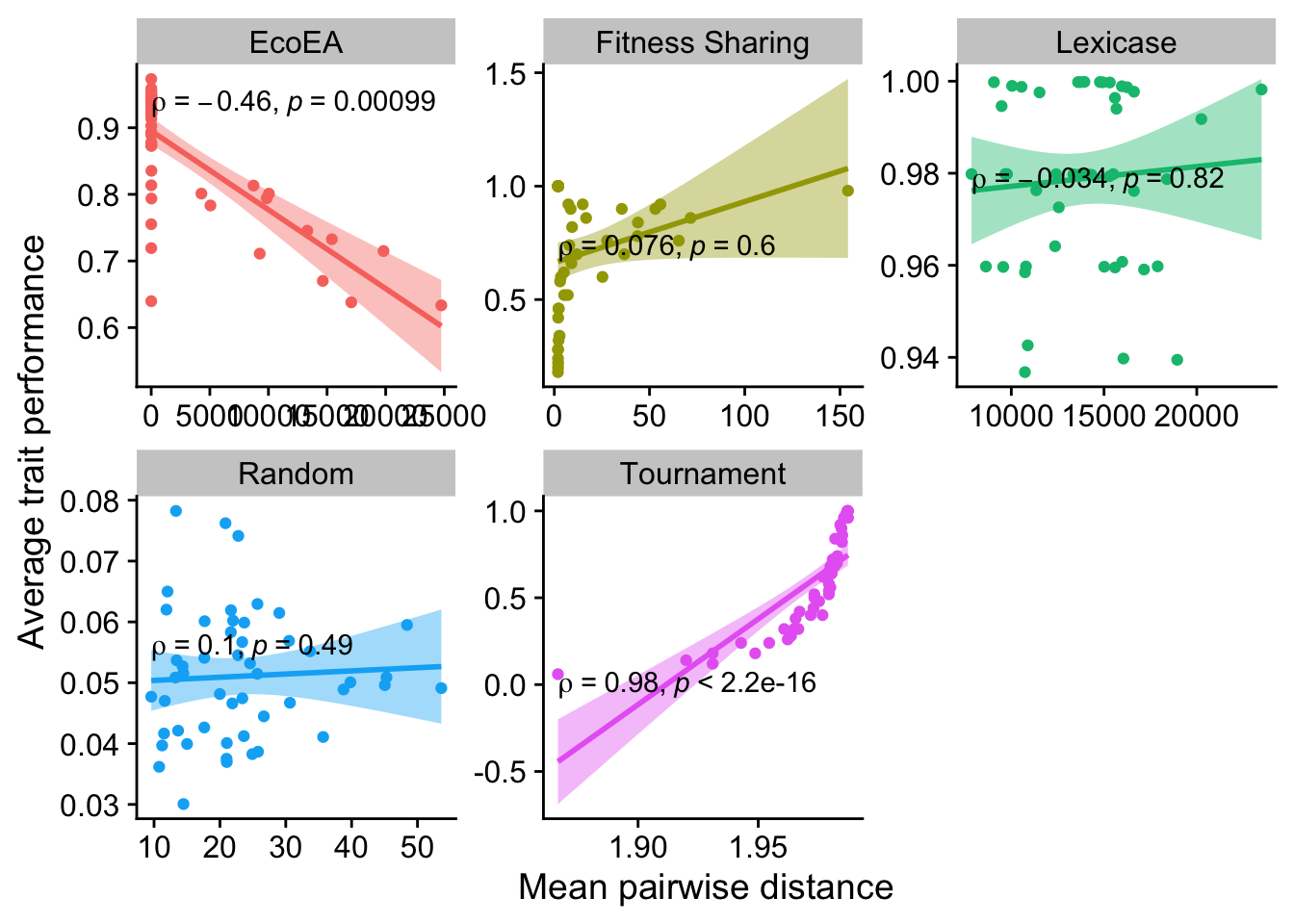

2.6.3.2 Mean evolutionary distinctiveness

ggplot(
    final_data,
    aes(
        y=elite_trait_avg,
        x=mean_phenotype_evolutionary_distinctiveness,
        color=selection_name,
        fill=selection_name
    )
  ) +
  geom_point() +
    scale_y_continuous(
        name="Average trait performance"
  ) +
  scale_x_continuous(
        name="Mean evolutionary distinctiveness"
  ) + 
  facet_wrap(
      ~selection_name, scales="free"
  ) + 
  stat_smooth(
    method="lm"
  ) + 
  stat_cor(
    method="spearman", cor.coef.name = "rho", color="black"
  ) +
  theme(legend.position = "none")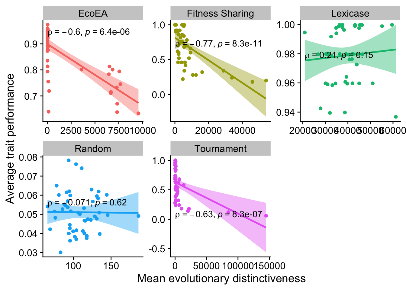

2.6.3.3 Richness

ggplot(
    final_data,
    aes(
        y=elite_trait_avg,
        x=phen_num_taxa,
        color=selection_name,
        fill=selection_name
    )
  ) +
  geom_point() +
    scale_y_continuous(
        name="Average trait performance"
  ) +
  scale_x_continuous(
        name="Phenotypic richness"
  ) + 
  facet_wrap(
      ~selection_name, scales="free"
  ) + 
  stat_smooth(
    method="lm"
  ) + 
  stat_cor(
    method="spearman", cor.coef.name = "rho", color="black"
  ) +
  theme(legend.position = "none")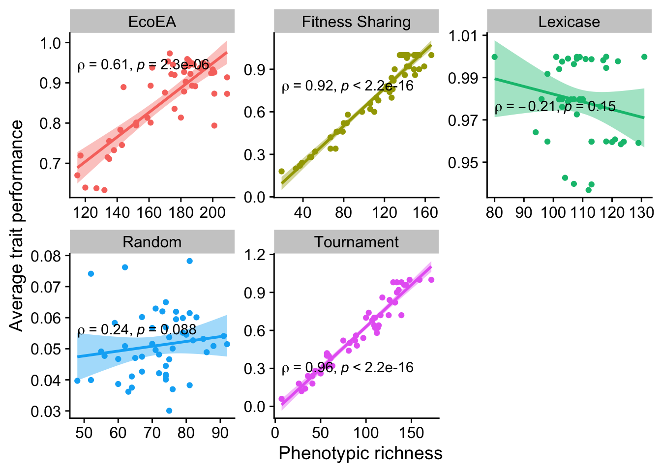

2.6.3.4 Shannon diversity

ggplot(
    final_data,
    aes(
        y=elite_trait_avg,
        x=phen_diversity,
        color=selection_name,
        fill=selection_name
    )
  ) +
  geom_point() +
    scale_y_continuous(
        name="Average trait performance"
  ) +
  scale_x_continuous(
        name="Phenotypic Shannon diversity"
  ) + 
  facet_wrap(
      ~selection_name, scales="free"
  ) + 
  stat_smooth(
    method="lm"
  ) + 
  stat_cor(
    method="spearman", cor.coef.name = "rho", color="black"
  ) +
  theme(legend.position = "none")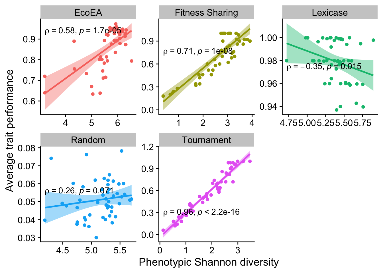

2.7 Causality analysis

Ultimately, it’s hard to draw useful inferences either from these single time point analyses or from comparison of line plots. Due to the feedbacks between diversity and performance, there may be a time delay in when one affects the other.

To analyze the drivers of this feedback loop in a more rigorous way, we turn to Transfer Entropy as a metric of Granger Causality. For a more thorough description, see the paper associated with this supplement.

2.7.1 Setup

First let’s define a function we’ll use to calculate and output significance and effect size for these results:

transfer_entropy_stats <- function(res) {
  stat.test <- res %>%
    group_by(selection_name, offset) %>%
    wilcox_test(value ~ Type) %>%
    adjust_pvalue(method = "bonferroni") %>%
    add_significance() 
  stat.test$label <- mapply(p_label,stat.test$p.adj)
  
  # Calculate effect sizes for these differences
  effect_sizes <- res %>%
    group_by(selection_name, offset) %>%
    wilcox_effsize(value ~ Type)
  
  stat.test$effsize <- effect_sizes$effsize
  stat.test$magnitude <- effect_sizes$magnitude
  
  stat.test %>%
    kbl() %>%
    kable_styling(
      bootstrap_options = c(
        "striped",
        "hover",
        "condensed",
        "responsive"
      )
    ) %>%
    scroll_box(width="600px")
}

2.7.2 Transfer entropy from diversity to fitness

First, we calculate the information that each type of diversity gives us about future fitness.

2.7.2.1 Max pairwise distance vs. phenotypic richness

We plot the differences in transfer entropy from phylogenetic diversity to fitness and from phenotypic diversity to fitness, at a range of different lags.

# Calculate transfer entropy for max pairwise distance
# Time points are 10 generations, so calculating lag 1 gives us lag 10
res <- data %>% group_by(directory, selection_name) %>%
summarise(
  fit_phylo_10 =     condinformation(discretize(elite_trait_avg), # TE phylo -> fit, lag 10
                                     discretize(lag(max_phenotype_pairwise_distance, 1)), 
                                     discretize(lag(elite_trait_avg, 1))),
  fit_phylo_100 =    condinformation(discretize(elite_trait_avg), # TE phylo -> fit, lag 100
                                     discretize(lag(max_phenotype_pairwise_distance, 10)), 
                                     discretize(lag(elite_trait_avg, 10))),
  fit_phylo_1000 =   condinformation(discretize(elite_trait_avg), # TE phylo -> fit, lag 1000
                                     discretize(lag(max_phenotype_pairwise_distance, 100)), 
                                     discretize(lag(elite_trait_avg, 100))),
  fit_phylo_10000 =  condinformation(discretize(elite_trait_avg), # TE phylo -> fit, lag 10000
                                     discretize(lag(max_phenotype_pairwise_distance, 1000)), 
                                     discretize(lag(elite_trait_avg, 1000))),
  fit_phylo_100000 = condinformation(discretize(elite_trait_avg), # TE phylo -> fit, lag 100000
                                     discretize(lag(max_phenotype_pairwise_distance, 10000)), 
                                     discretize(lag(elite_trait_avg, 10000))),  
  fit_fit_10000 =    condinformation(discretize(elite_trait_avg), # Mutual info btwn. fit and lagged fit
                                     discretize(lag(elite_trait_avg, 1000)), 
                                     discretize(lag(max_phenotype_pairwise_distance, 1000))),
  fit_fit_100000 =   condinformation(discretize(elite_trait_avg), # Mutual info btwn. fit and lagged fit
                                     discretize(lag(elite_trait_avg, 10000)), 
                                     discretize(lag(max_phenotype_pairwise_distance, 10000))),  
  fit_pheno_10 =     condinformation(discretize(elite_trait_avg), # TE pheno -> fit, lag 10
                                     discretize(lag(phen_num_taxa, 1)), 
                                     discretize(lag(elite_trait_avg, 1))),
  fit_pheno_100 =    condinformation(discretize(elite_trait_avg),  # TE pheno -> fit, lag 100 
                                     discretize(lag(phen_num_taxa, 10)), 
                                     discretize(lag(elite_trait_avg, 10))),
  fit_pheno_1000 =   condinformation(discretize(elite_trait_avg),  # TE pheno -> fit, lag 1000
                                     discretize(lag(phen_num_taxa, 100)), 
                                     discretize(lag(elite_trait_avg, 100))),
  fit_pheno_10000 =  condinformation(discretize(elite_trait_avg),  # TE pheno -> fit, lag 10000
                                     discretize(lag(phen_num_taxa, 1000)), 
                                     discretize(lag(elite_trait_avg, 1000))),
  fit_pheno_100000 = condinformation(discretize(elite_trait_avg),  # TE pheno -> fit, lag 100000
                                     discretize(lag(phen_num_taxa, 10000)), 
                                     discretize(lag(elite_trait_avg, 10000)))
)

# Turn Transfer Entropy columns into rows
res <- res %>% pivot_longer(cols=contains("o_10"))
# Pull lag into a column
res$offset <- str_extract(res$name, "[:digit:]*$")
# Make column indicating direction of transfer entropy
res$Type <- case_when(str_detect(res$name, "phylo") ~ "Phylogenetic", TRUE ~ "Phenotypic")

# Plot transfer entropy
ggplot(
  res %>% filter(str_detect(name, "fit_ph*")), 
  aes(
    x=as.factor(offset), 
    y=value, 
    color=Type
    )
  ) + 
  geom_boxplot() + 
  facet_wrap(~selection_name) + 
  scale_x_discrete("Lag",labels=c("10","","1000","","100000")) + 
  scale_y_continuous("Transfer Entropy") + 
  theme(legend.position = c(1, 0),
        legend.justification = c(1, 0)) + 
  scale_color_discrete("")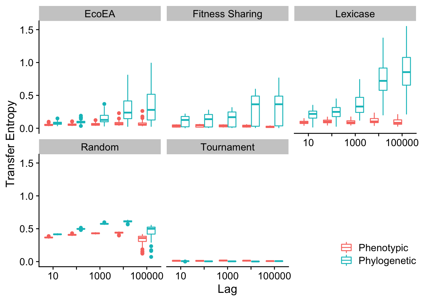

Next we calculate statistics to quantify these differences

# Determine which conditions are significantly different from each other
transfer_entropy_stats(res)

selection_name	offset	.y.	group1	group2	n1	n2	statistic	p	p.adj	p.adj.signif	label	effsize	magnitude
EcoEA	10	value	Phenotypic	Phylogenetic	50	50	466	1.00e-07	0.0000017	****	p < 1e-04	0.5404755	large
EcoEA	100	value	Phenotypic	Phylogenetic	50	50	234	0.00e+00	0.0000000	****	p < 1e-04	0.7004121	large
EcoEA	1000	value	Phenotypic	Phylogenetic	50	50	192	0.00e+00	0.0000000	****	p < 1e-04	0.7293661	large
EcoEA	10000	value	Phenotypic	Phylogenetic	50	50	165	0.00e+00	0.0000000	****	p < 1e-04	0.7479795	large
EcoEA	100000	value	Phenotypic	Phylogenetic	50	50	242	0.00e+00	0.0000000	****	p < 1e-04	0.6948970	large
Fitness Sharing	10	value	Phenotypic	Phylogenetic	50	50	798	1.85e-03	0.0462500		p = 0.04625	0.3116007	moderate
Fitness Sharing	100	value	Phenotypic	Phylogenetic	50	50	759	7.21e-04	0.0180250		p = 0.018025	0.3384866	moderate
Fitness Sharing	1000	value	Phenotypic	Phylogenetic	50	50	826	3.51e-03	0.0877500	ns	p = 0.08775	0.2922980	small
Fitness Sharing	10000	value	Phenotypic	Phylogenetic	50	50	661	4.97e-05	0.0012425	**	p = 0.0012425	0.4060460	moderate
Fitness Sharing	100000	value	Phenotypic	Phylogenetic	50	50	436	0.00e+00	0.0000005	****	p < 1e-04	0.5611569	large
Lexicase	10	value	Phenotypic	Phylogenetic	50	50	195	0.00e+00	0.0000000	****	p < 1e-04	0.7272980	large
Lexicase	100	value	Phenotypic	Phylogenetic	50	50	173	0.00e+00	0.0000000	****	p < 1e-04	0.7424644	large
Lexicase	1000	value	Phenotypic	Phylogenetic	50	50	34	0.00e+00	0.0000000	****	p < 1e-04	0.8382885	large
Lexicase	10000	value	Phenotypic	Phylogenetic	50	50	6	0.00e+00	0.0000000	****	p < 1e-04	0.8575912	large
Lexicase	100000	value	Phenotypic	Phylogenetic	50	50	1	0.00e+00	0.0000000	****	p < 1e-04	0.8610381	large
Random	10	value	Phenotypic	Phylogenetic	50	50	0	0.00e+00	0.0000000	****	p < 1e-04	0.8617275	large
Random	100	value	Phenotypic	Phylogenetic	50	50	0	0.00e+00	0.0000000	****	p < 1e-04	0.8617275	large
Random	1000	value	Phenotypic	Phylogenetic	50	50	0	0.00e+00	0.0000000	****	p < 1e-04	0.8617275	large
Random	10000	value	Phenotypic	Phylogenetic	50	50	0	0.00e+00	0.0000000	****	p < 1e-04	0.8617275	large
Random	100000	value	Phenotypic	Phylogenetic	50	50	358	0.00e+00	0.0000000	****	p < 1e-04	0.6149287	large
Tournament	10	value	Phenotypic	Phylogenetic	50	50	1810	1.15e-04	0.0028750	**	p = 0.002875	0.3860539	moderate
Tournament	100	value	Phenotypic	Phylogenetic	50	50	2024	1.00e-07	0.0000024	****	p < 1e-04	0.5335817	large
Tournament	1000	value	Phenotypic	Phylogenetic	50	50	2165	0.00e+00	0.0000000	****	p < 1e-04	0.6307845	large
Tournament	10000	value	Phenotypic	Phylogenetic	50	50	2322	0.00e+00	0.0000000	****	p < 1e-04	0.7390175	large
Tournament	100000	value	Phenotypic	Phylogenetic	50	50	1336	5.56e-01	1.0000000	ns	p = 1	0.0592869	small

2.7.2.2 Mean pairwise distance vs. phenotypic richness

# Calculate transfer entropy for mean pairwise distance
# Time points are 10 generations, so calculating lag 1 gives us lag 10
res <- data %>% group_by(directory, selection_name) %>%
summarise(
  fit_phylo_10 =     condinformation(discretize(elite_trait_avg), # TE phylo -> fit, lag 10
                                     discretize(lag(mean_phenotype_pairwise_distance, 1)), 
                                     discretize(lag(elite_trait_avg, 1))),
  fit_phylo_100 =    condinformation(discretize(elite_trait_avg), # TE phylo -> fit, lag 100
                                     discretize(lag(mean_phenotype_pairwise_distance, 10)), 
                                     discretize(lag(elite_trait_avg, 10))),
  fit_phylo_1000 =   condinformation(discretize(elite_trait_avg), # TE phylo -> fit, lag 1000
                                     discretize(lag(mean_phenotype_pairwise_distance, 100)), 
                                     discretize(lag(elite_trait_avg, 100))),
  fit_phylo_10000 =  condinformation(discretize(elite_trait_avg), # TE phylo -> fit, lag 10000
                                     discretize(lag(mean_phenotype_pairwise_distance, 1000)), 
                                     discretize(lag(elite_trait_avg, 1000))),
  fit_phylo_100000 = condinformation(discretize(elite_trait_avg), # TE phylo -> fit, lag 100000
                                     discretize(lag(mean_phenotype_pairwise_distance, 10000)), 
                                     discretize(lag(elite_trait_avg, 10000))),  
  fit_fit_10000 =    condinformation(discretize(elite_trait_avg), # Mutual info btwn. fit and lagged fit
                                     discretize(lag(elite_trait_avg, 1000)), 
                                     discretize(lag(mean_phenotype_pairwise_distance, 1000))),
  fit_fit_100000 =   condinformation(discretize(elite_trait_avg), # Mutual info btwn. fit and lagged fit
                                     discretize(lag(elite_trait_avg, 10000)), 
                                     discretize(lag(mean_phenotype_pairwise_distance, 10000))),  
  fit_pheno_10 =     condinformation(discretize(elite_trait_avg), # TE pheno -> fit, lag 10
                                     discretize(lag(phen_num_taxa, 1)), 
                                     discretize(lag(elite_trait_avg, 1))),
  fit_pheno_100 =    condinformation(discretize(elite_trait_avg),  # TE pheno -> fit, lag 100 
                                     discretize(lag(phen_num_taxa, 10)), 
                                     discretize(lag(elite_trait_avg, 10))),
  fit_pheno_1000 =   condinformation(discretize(elite_trait_avg),  # TE pheno -> fit, lag 1000
                                     discretize(lag(phen_num_taxa, 100)), 
                                     discretize(lag(elite_trait_avg, 100))),
  fit_pheno_10000 =  condinformation(discretize(elite_trait_avg),  # TE pheno -> fit, lag 10000
                                     discretize(lag(phen_num_taxa, 1000)), 
                                     discretize(lag(elite_trait_avg, 1000))),
  fit_pheno_100000 = condinformation(discretize(elite_trait_avg),  # TE pheno -> fit, lag 100000
                                     discretize(lag(phen_num_taxa, 10000)), 
                                     discretize(lag(elite_trait_avg, 10000)))
)

# Turn Transfer Entropy columns into rows
res <- res %>% pivot_longer(cols=contains("o_10"))
# Pull lag into a column
res$offset <- str_extract(res$name, "[:digit:]*$")
# Make column indicating direction of transfer entropy
res$Type <- case_when(str_detect(res$name, "phylo") ~ "Phylogenetic", TRUE ~ "Phenotypic")

# Plot transfer entropy
ggplot(
  res %>% filter(str_detect(name, "fit_ph*")), 
  aes(
    x=as.factor(offset), 
    y=value, 
    color=Type
    )
  ) + 
  geom_boxplot() + 
  facet_wrap(~selection_name) + 
  scale_x_discrete("Lag",labels=c("10","","1000","","100000")) + 
  scale_y_continuous("Transfer Entropy") + 
  theme(legend.position = c(1, 0),
        legend.justification = c(1, 0)) + 
  scale_color_discrete("")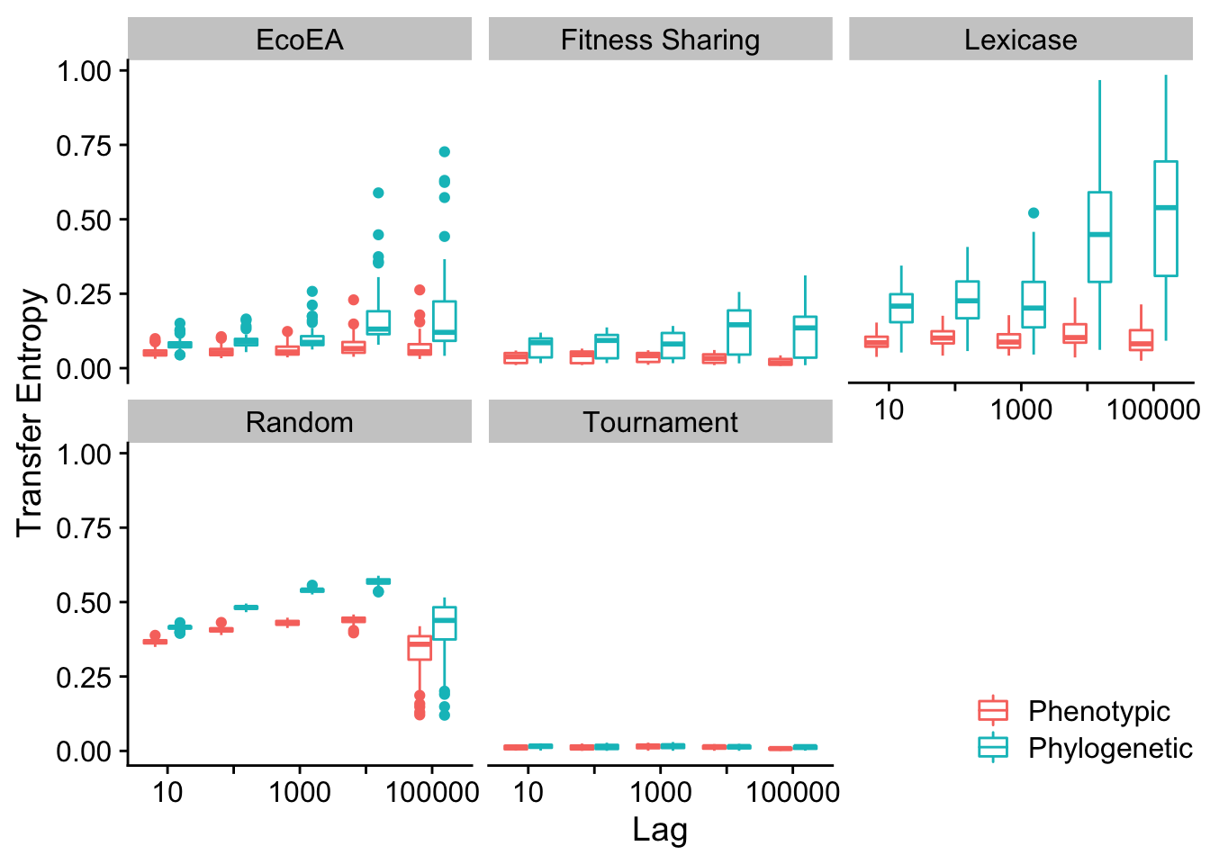

Mean and max pairwise distance appear to behave virtually identically.

# Determine which conditions are significantly different from each other
transfer_entropy_stats(res)

selection_name	offset	.y.	group1	group2	n1	n2	statistic	p	p.adj	p.adj.signif	label	effsize	magnitude
EcoEA	10	value	Phenotypic	Phylogenetic	50	50	288	0.00e+00	0.0000000	****	p < 1e-04	0.6631855	large
EcoEA	100	value	Phenotypic	Phylogenetic	50	50	256	0.00e+00	0.0000000	****	p < 1e-04	0.6852457	large
EcoEA	1000	value	Phenotypic	Phylogenetic	50	50	330	0.00e+00	0.0000000	****	p < 1e-04	0.6342314	large
EcoEA	10000	value	Phenotypic	Phylogenetic	50	50	209	0.00e+00	0.0000000	****	p < 1e-04	0.7176466	large
EcoEA	100000	value	Phenotypic	Phylogenetic	50	50	381	0.00e+00	0.0000001	****	p < 1e-04	0.5990729	large
Fitness Sharing	10	value	Phenotypic	Phylogenetic	50	50	521	5.00e-07	0.0000128	****	p < 1e-04	0.5025595	large
Fitness Sharing	100	value	Phenotypic	Phylogenetic	50	50	550	1.40e-06	0.0000355	****	p < 1e-04	0.4825674	moderate
Fitness Sharing	1000	value	Phenotypic	Phylogenetic	50	50	612	1.11e-05	0.0002775	***	p = 0.0002775	0.4398257	moderate
Fitness Sharing	10000	value	Phenotypic	Phylogenetic	50	50	459	1.00e-07	0.0000013	****	p < 1e-04	0.5453012	large
Fitness Sharing	100000	value	Phenotypic	Phylogenetic	50	50	350	0.00e+00	0.0000000	****	p < 1e-04	0.6204438	large
Lexicase	10	value	Phenotypic	Phylogenetic	50	50	195	0.00e+00	0.0000000	****	p < 1e-04	0.7272980	large
Lexicase	100	value	Phenotypic	Phylogenetic	50	50	220	0.00e+00	0.0000000	****	p < 1e-04	0.7100634	large
Lexicase	1000	value	Phenotypic	Phylogenetic	50	50	333	0.00e+00	0.0000000	****	p < 1e-04	0.6321633	large
Lexicase	10000	value	Phenotypic	Phylogenetic	50	50	142	0.00e+00	0.0000000	****	p < 1e-04	0.7638352	large
Lexicase	100000	value	Phenotypic	Phylogenetic	50	50	115	0.00e+00	0.0000000	****	p < 1e-04	0.7824486	large
Random	10	value	Phenotypic	Phylogenetic	50	50	0	0.00e+00	0.0000000	****	p < 1e-04	0.8617275	large
Random	100	value	Phenotypic	Phylogenetic	50	50	0	0.00e+00	0.0000000	****	p < 1e-04	0.8617275	large
Random	1000	value	Phenotypic	Phylogenetic	50	50	0	0.00e+00	0.0000000	****	p < 1e-04	0.8617275	large
Random	10000	value	Phenotypic	Phylogenetic	50	50	0	0.00e+00	0.0000000	****	p < 1e-04	0.8617275	large
Random	100000	value	Phenotypic	Phylogenetic	50	50	538	9.00e-07	0.0000233	****	p < 1e-04	0.4908400	moderate
Tournament	10	value	Phenotypic	Phylogenetic	50	50	928	2.67e-02	0.6675000	ns	p = 0.6675	0.2219810	small
Tournament	100	value	Phenotypic	Phylogenetic	50	50	1105	3.19e-01	1.0000000	ns	p = 1	0.0999604	small
Tournament	1000	value	Phenotypic	Phylogenetic	50	50	1184	6.52e-01	1.0000000	ns	p = 1	0.0454992	small
Tournament	10000	value	Phenotypic	Phylogenetic	50	50	1188	6.72e-01	1.0000000	ns	p = 1	0.0427417	small
Tournament	100000	value	Phenotypic	Phylogenetic	50	50	618	1.34e-05	0.0003350	***	p = 0.000335	0.4356894	moderate

2.7.2.3 Mean pairwise distance vs. shannon entropy

# Calculate transfer entropy for mean pairwise distance
# Time points are 10 generations, so calculating lag 1 gives us lag 10
res <- data %>% group_by(directory, selection_name) %>%
summarise(
  fit_phylo_10 =     condinformation(discretize(elite_trait_avg), # TE phylo -> fit, lag 10
                                     discretize(lag(mean_phenotype_pairwise_distance, 1)), 
                                     discretize(lag(elite_trait_avg, 1))),
  fit_phylo_100 =    condinformation(discretize(elite_trait_avg), # TE phylo -> fit, lag 100
                                     discretize(lag(mean_phenotype_pairwise_distance, 10)), 
                                     discretize(lag(elite_trait_avg, 10))),
  fit_phylo_1000 =   condinformation(discretize(elite_trait_avg), # TE phylo -> fit, lag 1000
                                     discretize(lag(mean_phenotype_pairwise_distance, 100)), 
                                     discretize(lag(elite_trait_avg, 100))),
  fit_phylo_10000 =  condinformation(discretize(elite_trait_avg), # TE phylo -> fit, lag 10000
                                     discretize(lag(mean_phenotype_pairwise_distance, 1000)), 
                                     discretize(lag(elite_trait_avg, 1000))),
  fit_phylo_100000 = condinformation(discretize(elite_trait_avg), # TE phylo -> fit, lag 100000
                                     discretize(lag(mean_phenotype_pairwise_distance, 10000)), 
                                     discretize(lag(elite_trait_avg, 10000))),  
  fit_fit_10000 =    condinformation(discretize(elite_trait_avg), # Mutual info btwn. fit and lagged fit
                                     discretize(lag(elite_trait_avg, 1000)), 
                                     discretize(lag(mean_phenotype_pairwise_distance, 1000))),
  fit_fit_100000 =   condinformation(discretize(elite_trait_avg), # Mutual info btwn. fit and lagged fit
                                     discretize(lag(elite_trait_avg, 10000)), 
                                     discretize(lag(mean_phenotype_pairwise_distance, 10000))),  
  fit_pheno_10 =     condinformation(discretize(elite_trait_avg), # TE pheno -> fit, lag 10
                                     discretize(lag(phen_diversity, 1)), 
                                     discretize(lag(elite_trait_avg, 1))),
  fit_pheno_100 =    condinformation(discretize(elite_trait_avg),  # TE pheno -> fit, lag 100 
                                     discretize(lag(phen_diversity, 10)), 
                                     discretize(lag(elite_trait_avg, 10))),
  fit_pheno_1000 =   condinformation(discretize(elite_trait_avg),  # TE pheno -> fit, lag 1000
                                     discretize(lag(phen_diversity, 100)), 
                                     discretize(lag(elite_trait_avg, 100))),
  fit_pheno_10000 =  condinformation(discretize(elite_trait_avg),  # TE pheno -> fit, lag 10000
                                     discretize(lag(phen_diversity, 1000)), 
                                     discretize(lag(elite_trait_avg, 1000))),
  fit_pheno_100000 = condinformation(discretize(elite_trait_avg),  # TE pheno -> fit, lag 100000
                                     discretize(lag(phen_diversity, 10000)), 
                                     discretize(lag(elite_trait_avg, 10000)))
)

# Turn Transfer Entropy columns into rows
res <- res %>% pivot_longer(cols=contains("o_10"))
# Pull lag into a column
res$offset <- str_extract(res$name, "[:digit:]*$")
# Make column indicating direction of transfer entropy
res$Type <- case_when(str_detect(res$name, "phylo") ~ "Phylogenetic", TRUE ~ "Phenotypic")

# Plot transfer entropy
ggplot(
  res %>% filter(str_detect(name, "fit_ph*")), 
  aes(
    x=as.factor(offset), 
    y=value, 
    color=Type
    )
  ) + 
  geom_boxplot() + 
  facet_wrap(~selection_name) + 
  scale_x_discrete("Lag",labels=c("10","","1000","","100000")) + 
  scale_y_continuous("Transfer Entropy") + 
  theme(legend.position = c(1, 0),
        legend.justification = c(1, 0)) + 
  scale_color_discrete("")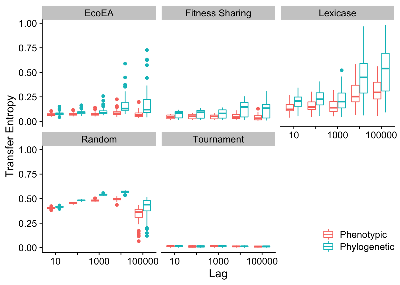

Looks like Shannon Diversity is more predictive of fitness than phenotypic richness (at least for lexicase), although still not as much as mean pairwise distance.

# Determine which conditions are significantly different from each other
transfer_entropy_stats(res)

selection_name	offset	.y.	group1	group2	n1	n2	statistic	p	p.adj	p.adj.signif	label	effsize	magnitude
EcoEA	10	value	Phenotypic	Phylogenetic	50	50	789	1.50e-03	0.0375000		p = 0.0375	0.3178051	moderate
EcoEA	100	value	Phenotypic	Phylogenetic	50	50	666	5.76e-05	0.0014400	**	p = 0.00144	0.4025991	moderate
EcoEA	1000	value	Phenotypic	Phylogenetic	50	50	678	8.15e-05	0.0020375	**	p = 0.0020375	0.3943265	moderate
EcoEA	10000	value	Phenotypic	Phylogenetic	50	50	291	0.00e+00	0.0000000	****	p < 1e-04	0.6611173	large
EcoEA	100000	value	Phenotypic	Phylogenetic	50	50	445	0.00e+00	0.0000007	****	p < 1e-04	0.5549525	large
Fitness Sharing	10	value	Phenotypic	Phylogenetic	50	50	706	1.79e-04	0.0044750	**	p = 0.004475	0.3750238	moderate
Fitness Sharing	100	value	Phenotypic	Phylogenetic	50	50	726	3.07e-04	0.0076750	**	p = 0.007675	0.3612362	moderate
Fitness Sharing	1000	value	Phenotypic	Phylogenetic	50	50	781	1.24e-03	0.0310000		p = 0.031	0.3233202	moderate
Fitness Sharing	10000	value	Phenotypic	Phylogenetic	50	50	617	1.30e-05	0.0003250	***	p = 0.000325	0.4363788	moderate
Fitness Sharing	100000	value	Phenotypic	Phylogenetic	50	50	538	9.00e-07	0.0000233	****	p < 1e-04	0.4908400	moderate
Lexicase	10	value	Phenotypic	Phylogenetic	50	50	561	2.10e-06	0.0000518	****	p < 1e-04	0.4749842	moderate
Lexicase	100	value	Phenotypic	Phylogenetic	50	50	612	1.11e-05	0.0002775	***	p = 0.0002775	0.4398257	moderate
Lexicase	1000	value	Phenotypic	Phylogenetic	50	50	829	3.75e-03	0.0937500	ns	p = 0.09375	0.2902298	small
Lexicase	10000	value	Phenotypic	Phylogenetic	50	50	610	1.04e-05	0.0002600	***	p = 0.00026	0.4412045	moderate
Lexicase	100000	value	Phenotypic	Phylogenetic	50	50	611	1.07e-05	0.0002675	***	p = 0.0002675	0.4405151	moderate
Random	10	value	Phenotypic	Phylogenetic	50	50	404	0.00e+00	0.0000001	****	p < 1e-04	0.5832172	large
Random	100	value	Phenotypic	Phylogenetic	50	50	1	0.00e+00	0.0000000	****	p < 1e-04	0.8610381	large
Random	1000	value	Phenotypic	Phylogenetic	50	50	0	0.00e+00	0.0000000	****	p < 1e-04	0.8617275	large
Random	10000	value	Phenotypic	Phylogenetic	50	50	0	0.00e+00	0.0000000	****	p < 1e-04	0.8617275	large
Random	100000	value	Phenotypic	Phylogenetic	50	50	580	3.90e-06	0.0000980	****	p < 1e-04	0.4618859	moderate
Tournament	10	value	Phenotypic	Phylogenetic	50	50	1241	9.53e-01	1.0000000	ns	p = 1	0.0062044	small
Tournament	100	value	Phenotypic	Phylogenetic	50	50	1225	8.66e-01	1.0000000	ns	p = 1	0.0172345	small
Tournament	1000	value	Phenotypic	Phylogenetic	50	50	1265	9.20e-01	1.0000000	ns	p = 1	0.0103407	small
Tournament	10000	value	Phenotypic	Phylogenetic	50	50	1217	8.23e-01	1.0000000	ns	p = 1	0.0227496	small
Tournament	100000	value	Phenotypic	Phylogenetic	50	50	1105	3.19e-01	1.0000000	ns	p = 1	0.0999604	small

2.7.2.4 Mean evolutionary distinctiveness vs. phenotypic richness

# Calculate transfer entropy for mean evolutionary distinctiveness
# Time points are 10 generations, so calculating lag 1 gives us lag 10
res <- data %>% group_by(directory, selection_name) %>%
summarise(
  fit_phylo_10 =     condinformation(discretize(elite_trait_avg), # TE phylo -> fit, lag 10
                                     discretize(lag(mean_phenotype_evolutionary_distinctiveness, 1)), 
                                     discretize(lag(elite_trait_avg, 1))),
  fit_phylo_100 =    condinformation(discretize(elite_trait_avg), # TE phylo -> fit, lag 100
                                     discretize(lag(mean_phenotype_evolutionary_distinctiveness, 10)), 
                                     discretize(lag(elite_trait_avg, 10))),
  fit_phylo_1000 =   condinformation(discretize(elite_trait_avg), # TE phylo -> fit, lag 1000
                                     discretize(lag(mean_phenotype_evolutionary_distinctiveness, 100)), 
                                     discretize(lag(elite_trait_avg, 100))),
  fit_phylo_10000 =  condinformation(discretize(elite_trait_avg), # TE phylo -> fit, lag 10000
                                     discretize(lag(mean_phenotype_evolutionary_distinctiveness, 1000)), 
                                     discretize(lag(elite_trait_avg, 1000))),
  fit_phylo_100000 = condinformation(discretize(elite_trait_avg), # TE phylo -> fit, lag 100000
                                     discretize(lag(mean_phenotype_evolutionary_distinctiveness, 10000)), 
                                     discretize(lag(elite_trait_avg, 10000))),  
  fit_fit_10000 =    condinformation(discretize(elite_trait_avg), # Mutual info btwn. fit and lagged fit
                                     discretize(lag(elite_trait_avg, 1000)), 
                                     discretize(lag(mean_phenotype_evolutionary_distinctiveness, 1000))),
  fit_fit_100000 =   condinformation(discretize(elite_trait_avg), # Mutual info btwn. fit and lagged fit
                                     discretize(lag(elite_trait_avg, 10000)), 
                                     discretize(lag(mean_phenotype_evolutionary_distinctiveness, 10000))),  
  fit_pheno_10 =     condinformation(discretize(elite_trait_avg), # TE pheno -> fit, lag 10
                                     discretize(lag(phen_num_taxa, 1)), 
                                     discretize(lag(elite_trait_avg, 1))),
  fit_pheno_100 =    condinformation(discretize(elite_trait_avg),  # TE pheno -> fit, lag 100 
                                     discretize(lag(phen_num_taxa, 10)), 
                                     discretize(lag(elite_trait_avg, 10))),
  fit_pheno_1000 =   condinformation(discretize(elite_trait_avg),  # TE pheno -> fit, lag 1000
                                     discretize(lag(phen_num_taxa, 100)), 
                                     discretize(lag(elite_trait_avg, 100))),
  fit_pheno_10000 =  condinformation(discretize(elite_trait_avg),  # TE pheno -> fit, lag 10000
                                     discretize(lag(phen_num_taxa, 1000)), 
                                     discretize(lag(elite_trait_avg, 1000))),
  fit_pheno_100000 = condinformation(discretize(elite_trait_avg),  # TE pheno -> fit, lag 100000
                                     discretize(lag(phen_num_taxa, 10000)), 
                                     discretize(lag(elite_trait_avg, 10000)))
)

# Turn Transfer Entropy columns into rows
res <- res %>% pivot_longer(cols=contains("o_10"))
# Pull lag into a column
res$offset <- str_extract(res$name, "[:digit:]*$")
# Make column indicating direction of transfer entropy
res$Type <- case_when(str_detect(res$name, "phylo") ~ "Phylogenetic", TRUE ~ "Phenotypic")

# Plot transfer entropy
ggplot(
  res %>% filter(str_detect(name, "fit_ph*")), 
  aes(
    x=as.factor(offset), 
    y=value, 
    color=Type
    )
  ) + 
  geom_boxplot() + 
  facet_wrap(~selection_name) + 
  scale_x_discrete("Lag",labels=c("10","","1000","","100000")) + 
  scale_y_continuous("Transfer Entropy") + 
  theme(legend.position = c(1, 0),
        legend.justification = c(1, 0)) + 
  scale_color_discrete("")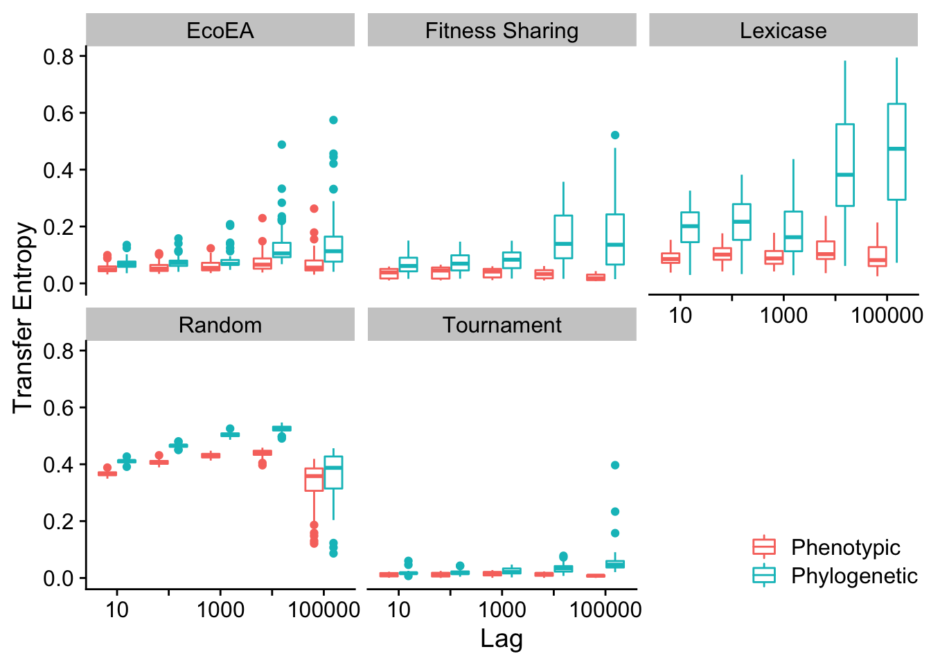

Interestingly, mean evolutionary distinctiveness looks fairly comparable to mean pairwise distance (although note that the y axis doesn’t go quite as far).

# Determine which conditions are significantly different from each other
transfer_entropy_stats(res)

selection_name	offset	.y.	group1	group2	n1	n2	statistic	p	p.adj	p.adj.signif	label	effsize	magnitude
EcoEA	10	value	Phenotypic	Phylogenetic	50	50	543	1.10e-06	0.0000278	****	p < 1e-04	0.4873931	moderate
EcoEA	100	value	Phenotypic	Phylogenetic	50	50	536	9.00e-07	0.0000218	****	p < 1e-04	0.4922187	moderate
EcoEA	1000	value	Phenotypic	Phylogenetic	50	50	644	2.99e-05	0.0007475	***	p = 0.0007475	0.4177655	moderate
EcoEA	10000	value	Phenotypic	Phylogenetic	50	50	380	0.00e+00	0.0000001	****	p < 1e-04	0.5997623	large
EcoEA	100000	value	Phenotypic	Phylogenetic	50	50	501	2.00e-07	0.0000062	****	p < 1e-04	0.5163471	large
Fitness Sharing	10	value	Phenotypic	Phylogenetic	50	50	531	7.00e-07	0.0000182	****	p < 1e-04	0.4956656	moderate
Fitness Sharing	100	value	Phenotypic	Phylogenetic	50	50	551	1.50e-06	0.0000368	****	p < 1e-04	0.4818780	moderate
Fitness Sharing	1000	value	Phenotypic	Phylogenetic	50	50	423	0.00e+00	0.0000003	****	p < 1e-04	0.5701189	large
Fitness Sharing	10000	value	Phenotypic	Phylogenetic	50	50	321	0.00e+00	0.0000000	****	p < 1e-04	0.6404359	large
Fitness Sharing	100000	value	Phenotypic	Phylogenetic	50	50	107	0.00e+00	0.0000000	****	p < 1e-04	0.7879636	large
Lexicase	10	value	Phenotypic	Phylogenetic	50	50	237	0.00e+00	0.0000000	****	p < 1e-04	0.6983440	large
Lexicase	100	value	Phenotypic	Phylogenetic	50	50	275	0.00e+00	0.0000000	****	p < 1e-04	0.6721474	large
Lexicase	1000	value	Phenotypic	Phylogenetic	50	50	516	4.00e-07	0.0000107	****	p < 1e-04	0.5060064	large
Lexicase	10000	value	Phenotypic	Phylogenetic	50	50	220	0.00e+00	0.0000000	****	p < 1e-04	0.7100634	large
Lexicase	100000	value	Phenotypic	Phylogenetic	50	50	178	0.00e+00	0.0000000	****	p < 1e-04	0.7390175	large
Random	10	value	Phenotypic	Phylogenetic	50	50	0	0.00e+00	0.0000000	****	p < 1e-04	0.8617275	large
Random	100	value	Phenotypic	Phylogenetic	50	50	0	0.00e+00	0.0000000	****	p < 1e-04	0.8617275	large
Random	1000	value	Phenotypic	Phylogenetic	50	50	0	0.00e+00	0.0000000	****	p < 1e-04	0.8617275	large
Random	10000	value	Phenotypic	Phylogenetic	50	50	0	0.00e+00	0.0000000	****	p < 1e-04	0.8617275	large
Random	100000	value	Phenotypic	Phylogenetic	50	50	893	1.40e-02	0.3500000	ns	p = 0.35	0.2461094	small
Tournament	10	value	Phenotypic	Phylogenetic	50	50	654	4.04e-05	0.0010100	**	p = 0.00101	0.4108717	moderate
Tournament	100	value	Phenotypic	Phylogenetic	50	50	718	2.48e-04	0.0062000	**	p = 0.0062	0.3667512	moderate
Tournament	1000	value	Phenotypic	Phylogenetic	50	50	735	3.90e-04	0.0097500	**	p = 0.00975	0.3550317	moderate
Tournament	10000	value	Phenotypic	Phylogenetic	50	50	180	0.00e+00	0.0000000	****	p < 1e-04	0.7376387	large
Tournament	100000	value	Phenotypic	Phylogenetic	50	50	0	0.00e+00	0.0000000	****	p < 1e-04	0.8617275	large

2.7.2.5 Mean evolutionary distinctiveness vs. shannon entropy

# Calculate transfer entropy for mean evolutionary distinctiveness
# Time points are 10 generations, so calculating lag 1 gives us lag 10
res <- data %>% group_by(directory, selection_name) %>%
summarise(
  fit_phylo_10 =     condinformation(discretize(elite_trait_avg), # TE phylo -> fit, lag 10
                                     discretize(lag(mean_phenotype_evolutionary_distinctiveness, 1)), 
                                     discretize(lag(elite_trait_avg, 1))),
  fit_phylo_100 =    condinformation(discretize(elite_trait_avg), # TE phylo -> fit, lag 100
                                     discretize(lag(mean_phenotype_evolutionary_distinctiveness, 10)), 
                                     discretize(lag(elite_trait_avg, 10))),
  fit_phylo_1000 =   condinformation(discretize(elite_trait_avg), # TE phylo -> fit, lag 1000
                                     discretize(lag(mean_phenotype_evolutionary_distinctiveness, 100)), 
                                     discretize(lag(elite_trait_avg, 100))),
  fit_phylo_10000 =  condinformation(discretize(elite_trait_avg), # TE phylo -> fit, lag 10000
                                     discretize(lag(mean_phenotype_evolutionary_distinctiveness, 1000)), 
                                     discretize(lag(elite_trait_avg, 1000))),
  fit_phylo_100000 = condinformation(discretize(elite_trait_avg), # TE phylo -> fit, lag 100000
                                     discretize(lag(mean_phenotype_evolutionary_distinctiveness, 10000)), 
                                     discretize(lag(elite_trait_avg, 10000))),  
  fit_fit_10000 =    condinformation(discretize(elite_trait_avg), # Mutual info btwn. fit and lagged fit
                                     discretize(lag(elite_trait_avg, 1000)), 
                                     discretize(lag(mean_phenotype_evolutionary_distinctiveness, 1000))),
  fit_fit_100000 =   condinformation(discretize(elite_trait_avg), # Mutual info btwn. fit and lagged fit
                                     discretize(lag(elite_trait_avg, 10000)), 
                                     discretize(lag(mean_phenotype_evolutionary_distinctiveness, 10000))),  
  fit_pheno_10 =     condinformation(discretize(elite_trait_avg), # TE pheno -> fit, lag 10
                                     discretize(lag(phen_diversity, 1)), 
                                     discretize(lag(elite_trait_avg, 1))),
  fit_pheno_100 =    condinformation(discretize(elite_trait_avg),  # TE pheno -> fit, lag 100 
                                     discretize(lag(phen_diversity, 10)), 
                                     discretize(lag(elite_trait_avg, 10))),
  fit_pheno_1000 =   condinformation(discretize(elite_trait_avg),  # TE pheno -> fit, lag 1000
                                     discretize(lag(phen_diversity, 100)), 
                                     discretize(lag(elite_trait_avg, 100))),
  fit_pheno_10000 =  condinformation(discretize(elite_trait_avg),  # TE pheno -> fit, lag 10000
                                     discretize(lag(phen_diversity, 1000)), 
                                     discretize(lag(elite_trait_avg, 1000))),
  fit_pheno_100000 = condinformation(discretize(elite_trait_avg),  # TE pheno -> fit, lag 100000
                                     discretize(lag(phen_diversity, 10000)), 
                                     discretize(lag(elite_trait_avg, 10000)))
)

# Turn Transfer Entropy columns into rows
res <- res %>% pivot_longer(cols=contains("o_10"))
# Pull lag into a column
res$offset <- str_extract(res$name, "[:digit:]*$")
# Make column indicating direction of transfer entropy
res$Type <- case_when(str_detect(res$name, "phylo") ~ "Phylogenetic", TRUE ~ "Phenotypic")

# Plot transfer entropy
ggplot(
  res %>% filter(str_detect(name, "fit_ph*")), 
  aes(
    x=as.factor(offset), 
    y=value, 
    color=Type
    )
  ) + 
  geom_boxplot() + 
  facet_wrap(~selection_name) + 
  scale_x_discrete("Lag",labels=c("10","","1000","","100000")) + 
  scale_y_continuous("Transfer Entropy") + 
  theme(legend.position = c(1, 0),
        legend.justification = c(1, 0)) + 
  scale_color_discrete("")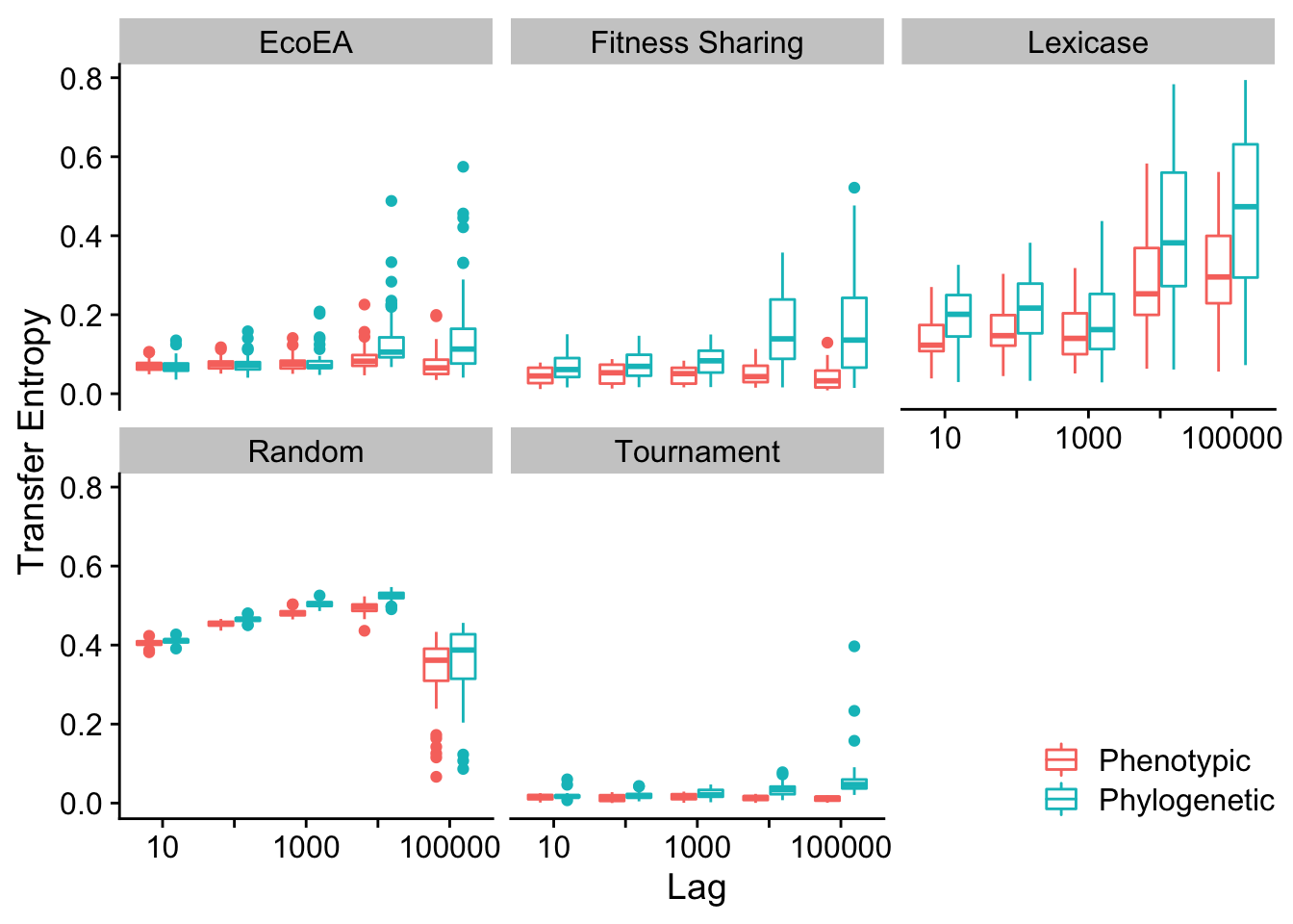

# Determine which conditions are significantly different from each other
transfer_entropy_stats(res)

selection_name	offset	.y.	group1	group2	n1	n2	statistic	p	p.adj	p.adj.signif	label	effsize	magnitude
EcoEA	10	value	Phenotypic	Phylogenetic	50	50	1381	3.68e-01	1.0000000	ns	p = 1	0.0903090	small
EcoEA	100	value	Phenotypic	Phylogenetic	50	50	1356	4.67e-01	1.0000000	ns	p = 1	0.0730745	small
EcoEA	1000	value	Phenotypic	Phylogenetic	50	50	1345	5.15e-01	1.0000000	ns	p = 1	0.0654913	small
EcoEA	10000	value	Phenotypic	Phylogenetic	50	50	527	6.00e-07	0.0000158	****	p < 1e-04	0.4984232	moderate
EcoEA	100000	value	Phenotypic	Phylogenetic	50	50	585	4.60e-06	0.0001158	***	p = 0.00011575	0.4584390	moderate
Fitness Sharing	10	value	Phenotypic	Phylogenetic	50	50	816	2.80e-03	0.0700000	ns	p = 0.07	0.2991918	small
Fitness Sharing	100	value	Phenotypic	Phylogenetic	50	50	839	4.66e-03	0.1165000	ns	p = 0.1165	0.2833360	small
Fitness Sharing	1000	value	Phenotypic	Phylogenetic	50	50	620	1.43e-05	0.0003575	***	p = 0.0003575	0.4343107	moderate
Fitness Sharing	10000	value	Phenotypic	Phylogenetic	50	50	452	0.00e+00	0.0000010	****	p < 1e-04	0.5501268	large
Fitness Sharing	100000	value	Phenotypic	Phylogenetic	50	50	328	0.00e+00	0.0000000	****	p < 1e-04	0.6356102	large
Lexicase	10	value	Phenotypic	Phylogenetic	50	50	644	2.99e-05	0.0007475	***	p = 0.0007475	0.4177655	moderate
Lexicase	100	value	Phenotypic	Phylogenetic	50	50	700	1.52e-04	0.0038000	**	p = 0.0038	0.3791601	moderate
Lexicase	1000	value	Phenotypic	Phylogenetic	50	50	1043	1.55e-01	1.0000000	ns	p = 1	0.1427021	small
Lexicase	10000	value	Phenotypic	Phylogenetic	50	50	766	8.59e-04	0.0214750		p = 0.021475	0.3336609	moderate
Lexicase	100000	value	Phenotypic	Phylogenetic	50	50	693	1.25e-04	0.0031250	**	p = 0.003125	0.3839858	moderate
Random	10	value	Phenotypic	Phylogenetic	50	50	718	2.48e-04	0.0062000	**	p = 0.0062	0.3667512	moderate
Random	100	value	Phenotypic	Phylogenetic	50	50	271	0.00e+00	0.0000000	****	p < 1e-04	0.6749050	large
Random	1000	value	Phenotypic	Phylogenetic	50	50	72	0.00e+00	0.0000000	****	p < 1e-04	0.8120920	large
Random	10000	value	Phenotypic	Phylogenetic	50	50	130	0.00e+00	0.0000000	****	p < 1e-04	0.7721078	large
Random	100000	value	Phenotypic	Phylogenetic	50	50	957	4.38e-02	1.0000000	ns	p = 1	0.2019889	small
Tournament	10	value	Phenotypic	Phylogenetic	50	50	1034	1.37e-01	1.0000000	ns	p = 1	0.1489065	small
Tournament	100	value	Phenotypic	Phylogenetic	50	50	867	8.37e-03	0.2092500	ns	p = 0.20925	0.2640333	small
Tournament	1000	value	Phenotypic	Phylogenetic	50	50	791	1.57e-03	0.0392500		p = 0.03925	0.3164263	moderate
Tournament	10000	value	Phenotypic	Phylogenetic	50	50	195	0.00e+00	0.0000000	****	p < 1e-04	0.7272980	large
Tournament	100000	value	Phenotypic	Phylogenetic	50	50	0	0.00e+00	0.0000000	****	p < 1e-04	0.8617275	large

2.7.3 Transfer entropy between types of diversity

While we’re calculating transfer entropy, we might as well also calculate it between phenotypic diversity and phylogenetic diversity, as these could potentially also be in a feedback loop.

2.7.3.1 Max pairwise distance and phenotypic richness

res <- data %>% group_by(directory, selection_name) %>%
summarise(
  phen_phylo_10 =      condinformation(discretize(phen_num_taxa), 
                                       discretize(lag(max_phenotype_pairwise_distance, 1)), 
                                       discretize(lag(phen_num_taxa, 1))),
  phen_phylo_100 =     condinformation(discretize(phen_num_taxa),
                                       discretize(lag(max_phenotype_pairwise_distance, 10)),
                                       discretize(lag(phen_num_taxa, 10))),
  pheno_phylo_1000 =   condinformation(discretize(phen_num_taxa),
                                       discretize(lag(max_phenotype_pairwise_distance, 100)),
                                       discretize(lag(phen_num_taxa, 100))),
  pheno_phylo_10000 =  condinformation(discretize(phen_num_taxa),
                                       discretize(lag(max_phenotype_pairwise_distance, 1000)),
                                       discretize(lag(phen_num_taxa, 1000))),
  pheno_phylo_100000 = condinformation(discretize(phen_num_taxa),
                                       discretize(lag(max_phenotype_pairwise_distance, 10000)),
                                       discretize(lag(phen_num_taxa, 10000))),
  
  phylo_pheno_10 =     condinformation(discretize(max_phenotype_pairwise_distance),
                                       discretize(lag(phen_num_taxa, 1)),
                                       discretize(lag(max_phenotype_pairwise_distance, 1))),
  phylo_pheno_100 =    condinformation(discretize(max_phenotype_pairwise_distance),
                                       discretize(lag(phen_num_taxa, 10)),
                                       discretize(lag(max_phenotype_pairwise_distance, 10))),
  phylo_pheno_1000 =   condinformation(discretize(max_phenotype_pairwise_distance),
                                       discretize(lag(phen_num_taxa, 100)),
                                       discretize(lag(max_phenotype_pairwise_distance, 100))),
  phylo_pheno_10000 =  condinformation(discretize(max_phenotype_pairwise_distance),
                                       discretize(lag(phen_num_taxa, 1000)),
                                       discretize(lag(max_phenotype_pairwise_distance, 1000))),
  phylo_pheno_100000 = condinformation(discretize(max_phenotype_pairwise_distance),
                                       discretize(lag(phen_num_taxa, 10000)),
                                       discretize(lag(max_phenotype_pairwise_distance, 10000)))
)

# Turn Transfer Entropy columns into rows
res <- res %>% pivot_longer(cols=contains("phylo"))
# Pull lag into a column
res$offset <- str_extract(res$name, "[:digit:]*$")
# Make column indicating direction of transfer entropy
res$Type <- case_when(str_detect(res$name, "phylo_pheno") ~ "\nPhenotypic\n\t->\nPhylogenetic\n", TRUE ~ "\nPhylogenetic\n\t->\nPhenotypic\n")

ggplot(
  res, 
  aes(
    x=as.factor(offset), 
    y=value, 
    color=Type
    )
  ) + 
  geom_boxplot() + 
  facet_wrap(~selection_name) + 
  scale_x_discrete("Lag",labels=c("10","","1000","","100000")) + 
  scale_y_continuous("Transfer Entropy") + 
  theme(legend.position = c(1, 0),
        legend.justification = c(1, 0)) + 
  scale_color_discrete("")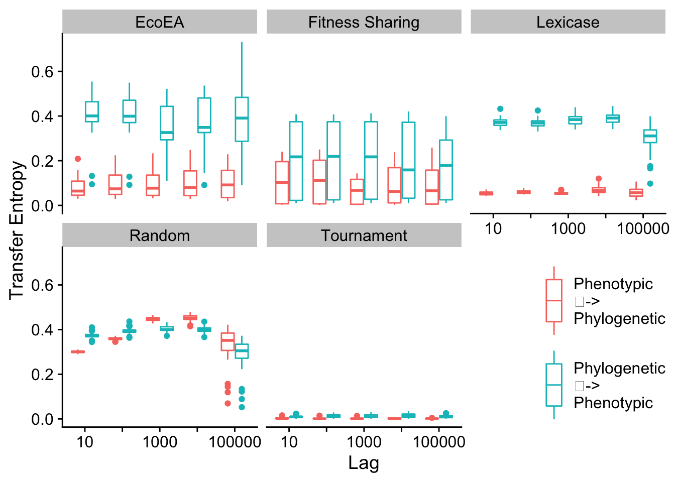

# Determine which conditions are significantly different from each other
transfer_entropy_stats(res)

selection_name	offset	.y.	group1	group2	n1	n2	statistic	p	p.adj	p.adj.signif	label	effsize	magnitude
EcoEA	10	value	Phenotypic -> Phylogenetic	Phylogenetic -> Phenotypic	50	50	23	0.00e+00	0.0000000	****	p < 1e-04	0.8458717	large
EcoEA	100	value	Phenotypic -> Phylogenetic	Phylogenetic -> Phenotypic	50	50	35	0.00e+00	0.0000000	****	p < 1e-04	0.8375991	large
EcoEA	1000	value	Phenotypic -> Phylogenetic	Phylogenetic -> Phenotypic	50	50	27	0.00e+00	0.0000000	****	p < 1e-04	0.8431142	large
EcoEA	10000	value	Phenotypic -> Phylogenetic	Phylogenetic -> Phenotypic	50	50	38	0.00e+00	0.0000000	****	p < 1e-04	0.8355310	large
EcoEA	100000	value	Phenotypic -> Phylogenetic	Phylogenetic -> Phenotypic	50	50	69	0.00e+00	0.0000000	****	p < 1e-04	0.8141601	large
Fitness Sharing	10	value	Phenotypic -> Phylogenetic	Phylogenetic -> Phenotypic	50	50	768	9.02e-04	0.0225500		p = 0.02255	0.3322821	moderate
Fitness Sharing	100	value	Phenotypic -> Phylogenetic	Phylogenetic -> Phenotypic	50	50	747	5.32e-04	0.0133000		p = 0.0133	0.3467591	moderate
Fitness Sharing	1000	value	Phenotypic -> Phylogenetic	Phylogenetic -> Phenotypic	50	50	666	5.76e-05	0.0014400	**	p = 0.00144	0.4025991	moderate
Fitness Sharing	10000	value	Phenotypic -> Phylogenetic	Phylogenetic -> Phenotypic	50	50	732	3.60e-04	0.0090000	**	p = 0.009	0.3570999	moderate
Fitness Sharing	100000	value	Phenotypic -> Phylogenetic	Phylogenetic -> Phenotypic	50	50	745	5.05e-04	0.0126250		p = 0.012625	0.3481379	moderate
Lexicase	10	value	Phenotypic -> Phylogenetic	Phylogenetic -> Phenotypic	50	50	0	0.00e+00	0.0000000	****	p < 1e-04	0.8617275	large
Lexicase	100	value	Phenotypic -> Phylogenetic	Phylogenetic -> Phenotypic	50	50	0	0.00e+00	0.0000000	****	p < 1e-04	0.8617275	large
Lexicase	1000	value	Phenotypic -> Phylogenetic	Phylogenetic -> Phenotypic	50	50	0	0.00e+00	0.0000000	****	p < 1e-04	0.8617275	large
Lexicase	10000	value	Phenotypic -> Phylogenetic	Phylogenetic -> Phenotypic	50	50	0	0.00e+00	0.0000000	****	p < 1e-04	0.8617275	large
Lexicase	100000	value	Phenotypic -> Phylogenetic	Phylogenetic -> Phenotypic	50	50	1	0.00e+00	0.0000000	****	p < 1e-04	0.8610381	large
Random	10	value	Phenotypic -> Phylogenetic	Phylogenetic -> Phenotypic	50	50	0	0.00e+00	0.0000000	****	p < 1e-04	0.8617275	large
Random	100	value	Phenotypic -> Phylogenetic	Phylogenetic -> Phenotypic	50	50	15	0.00e+00	0.0000000	****	p < 1e-04	0.8513868	large
Random	1000	value	Phenotypic -> Phylogenetic	Phylogenetic -> Phenotypic	50	50	2497	0.00e+00	0.0000000	****	p < 1e-04	0.8596593	large
Random	10000	value	Phenotypic -> Phylogenetic	Phylogenetic -> Phenotypic	50	50	2479	0.00e+00	0.0000000	****	p < 1e-04	0.8472505	large
Random	100000	value	Phenotypic -> Phylogenetic	Phylogenetic -> Phenotypic	50	50	1849	3.69e-05	0.0009225	***	p = 0.0009225	0.4129398	moderate
Tournament	10	value	Phenotypic -> Phylogenetic	Phylogenetic -> Phenotypic	50	50	168	0.00e+00	0.0000000	****	p < 1e-04	0.7459113	large
Tournament	100	value	Phenotypic -> Phylogenetic	Phylogenetic -> Phenotypic	50	50	53	0.00e+00	0.0000000	****	p < 1e-04	0.8251902	large
Tournament	1000	value	Phenotypic -> Phylogenetic	Phylogenetic -> Phenotypic	50	50	74	0.00e+00	0.0000000	****	p < 1e-04	0.8107132	large
Tournament	10000	value	Phenotypic -> Phylogenetic	Phylogenetic -> Phenotypic	50	50	60	0.00e+00	0.0000000	****	p < 1e-04	0.8203646	large
Tournament	100000	value	Phenotypic -> Phylogenetic	Phylogenetic -> Phenotypic	50	50	115	0.00e+00	0.0000000	****	p < 1e-04	0.7824486	large

2.7.3.2 Mean pairwise distance and phenotypic richness

res <- data %>% group_by(directory, selection_name) %>%
summarise(
  phen_phylo_10 =      condinformation(discretize(phen_num_taxa), 
                                       discretize(lag(mean_phenotype_pairwise_distance, 1)), 
                                       discretize(lag(phen_num_taxa, 1))),
  phen_phylo_100 =     condinformation(discretize(phen_num_taxa),
                                       discretize(lag(mean_phenotype_pairwise_distance, 10)),
                                       discretize(lag(phen_num_taxa, 10))),
  pheno_phylo_1000 =   condinformation(discretize(phen_num_taxa),
                                       discretize(lag(mean_phenotype_pairwise_distance, 100)),
                                       discretize(lag(phen_num_taxa, 100))),
  pheno_phylo_10000 =  condinformation(discretize(phen_num_taxa),
                                       discretize(lag(mean_phenotype_pairwise_distance, 1000)),
                                       discretize(lag(phen_num_taxa, 1000))),
  pheno_phylo_100000 = condinformation(discretize(phen_num_taxa),
                                       discretize(lag(mean_phenotype_pairwise_distance, 10000)),
                                       discretize(lag(phen_num_taxa, 10000))),
  
  phylo_pheno_10 =     condinformation(discretize(mean_phenotype_pairwise_distance),
                                       discretize(lag(phen_num_taxa, 1)),
                                       discretize(lag(mean_phenotype_pairwise_distance, 1))),
  phylo_pheno_100 =    condinformation(discretize(mean_phenotype_pairwise_distance),
                                       discretize(lag(phen_num_taxa, 10)),
                                       discretize(lag(mean_phenotype_pairwise_distance, 10))),
  phylo_pheno_1000 =   condinformation(discretize(mean_phenotype_pairwise_distance),
                                       discretize(lag(phen_num_taxa, 100)),
                                       discretize(lag(mean_phenotype_pairwise_distance, 100))),
  phylo_pheno_10000 =  condinformation(discretize(mean_phenotype_pairwise_distance),
                                       discretize(lag(phen_num_taxa, 1000)),
                                       discretize(lag(mean_phenotype_pairwise_distance, 1000))),
  phylo_pheno_100000 = condinformation(discretize(mean_phenotype_pairwise_distance),
                                       discretize(lag(phen_num_taxa, 10000)),
                                       discretize(lag(mean_phenotype_pairwise_distance, 10000)))
)

# Turn Transfer Entropy columns into rows
res <- res %>% pivot_longer(cols=contains("phylo"))
# Pull lag into a column
res$offset <- str_extract(res$name, "[:digit:]*$")
# Make column indicating direction of transfer entropy
res$Type <- case_when(str_detect(res$name, "phylo_pheno") ~ "\nPhenotypic\n\t->\nPhylogenetic\n", TRUE ~ "\nPhylogenetic\n\t->\nPhenotypic\n")

ggplot(
  res, 
  aes(
    x=as.factor(offset), 
    y=value, 
    color=Type
    )
  ) + 
  geom_boxplot() + 
  facet_wrap(~selection_name) + 
  scale_x_discrete("Lag",labels=c("10","","1000","","100000")) + 
  scale_y_continuous("Transfer Entropy") + 
  theme(legend.position = c(1, 0),
        legend.justification = c(1, 0)) + 
  scale_color_discrete("")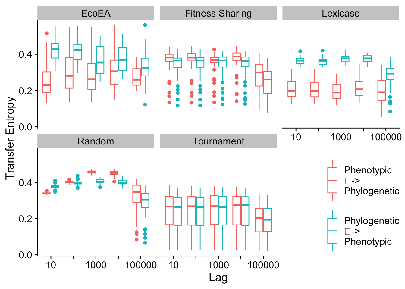

Here, on the other hand, there’s a pretty notable difference between mean and max pairwise distance. Looks like max pairwise distance is in general more predictive of phenotypic richness than mean pairwise distance is (for fitness sharing, mean richness even has a high transfer entropy to MPD than the other way around).

# Determine which conditions are significantly different from each other
transfer_entropy_stats(res)

selection_name	offset	.y.	group1	group2	n1	n2	statistic	p	p.adj	p.adj.signif	label	effsize	magnitude
EcoEA	10	value	Phenotypic -> Phylogenetic	Phylogenetic -> Phenotypic	50	50	342	0.00e+00	0.0000000	****	p < 1e-04	0.6259588	large
EcoEA	100	value	Phenotypic -> Phylogenetic	Phylogenetic -> Phenotypic	50	50	488	2.00e-07	0.0000038	****	p < 1e-04	0.5253091	large
EcoEA	1000	value	Phenotypic -> Phylogenetic	Phylogenetic -> Phenotypic	50	50	661	4.97e-05	0.0012425	**	p = 0.0012425	0.4060460	moderate
EcoEA	10000	value	Phenotypic -> Phylogenetic	Phylogenetic -> Phenotypic	50	50	720	2.62e-04	0.0065500	**	p = 0.00655	0.3653725	moderate
EcoEA	100000	value	Phenotypic -> Phylogenetic	Phylogenetic -> Phenotypic	50	50	735	3.90e-04	0.0097500	**	p = 0.00975	0.3550317	moderate
Fitness Sharing	10	value	Phenotypic -> Phylogenetic	Phylogenetic -> Phenotypic	50	50	1602	1.54e-02	0.3850000	ns	p = 0.385	0.2426625	small
Fitness Sharing	100	value	Phenotypic -> Phylogenetic	Phylogenetic -> Phenotypic	50	50	1653	5.52e-03	0.1380000	ns	p = 0.138	0.2778209	small
Fitness Sharing	1000	value	Phenotypic -> Phylogenetic	Phylogenetic -> Phenotypic	50	50	1369	4.14e-01	1.0000000	ns	p = 1	0.0820365	small
Fitness Sharing	10000	value	Phenotypic -> Phylogenetic	Phylogenetic -> Phenotypic	50	50	1744	6.69e-04	0.0167250		p = 0.016725	0.3405547	moderate
Fitness Sharing	100000	value	Phenotypic -> Phylogenetic	Phylogenetic -> Phenotypic	50	50	1571	2.71e-02	0.6775000	ns	p = 0.6775	0.2212916	small
Lexicase	10	value	Phenotypic -> Phylogenetic	Phylogenetic -> Phenotypic	50	50	0	0.00e+00	0.0000000	****	p < 1e-04	0.8617275	large
Lexicase	100	value	Phenotypic -> Phylogenetic	Phylogenetic -> Phenotypic	50	50	0	0.00e+00	0.0000000	****	p < 1e-04	0.8617275	large
Lexicase	1000	value	Phenotypic -> Phylogenetic	Phylogenetic -> Phenotypic	50	50	0	0.00e+00	0.0000000	****	p < 1e-04	0.8617275	large
Lexicase	10000	value	Phenotypic -> Phylogenetic	Phylogenetic -> Phenotypic	50	50	4	0.00e+00	0.0000000	****	p < 1e-04	0.8589700	large
Lexicase	100000	value	Phenotypic -> Phylogenetic	Phylogenetic -> Phenotypic	50	50	409	0.00e+00	0.0000002	****	p < 1e-04	0.5797703	large
Random	10	value	Phenotypic -> Phylogenetic	Phylogenetic -> Phenotypic	50	50	2	0.00e+00	0.0000000	****	p < 1e-04	0.8603487	large
Random	100	value	Phenotypic -> Phylogenetic	Phylogenetic -> Phenotypic	50	50	1771	3.33e-04	0.0083250	**	p = 0.008325	0.3591680	moderate
Random	1000	value	Phenotypic -> Phylogenetic	Phylogenetic -> Phenotypic	50	50	2500	0.00e+00	0.0000000	****	p < 1e-04	0.8617275	large
Random	10000	value	Phenotypic -> Phylogenetic	Phylogenetic -> Phenotypic	50	50	2473	0.00e+00	0.0000000	****	p < 1e-04	0.8431142	large
Random	100000	value	Phenotypic -> Phylogenetic	Phylogenetic -> Phenotypic	50	50	1749	5.89e-04	0.0147250		p = 0.014725	0.3440016	moderate
Tournament	10	value	Phenotypic -> Phylogenetic	Phylogenetic -> Phenotypic	50	50	1298	7.43e-01	1.0000000	ns	p = 1	0.0330903	small
Tournament	100	value	Phenotypic -> Phylogenetic	Phylogenetic -> Phenotypic	50	50	1306	7.02e-01	1.0000000	ns	p = 1	0.0386054	small
Tournament	1000	value	Phenotypic -> Phylogenetic	Phylogenetic -> Phenotypic	50	50	1301	7.28e-01	1.0000000	ns	p = 1	0.0351585	small
Tournament	10000	value	Phenotypic -> Phylogenetic	Phylogenetic -> Phenotypic	50	50	1276	8.60e-01	1.0000000	ns	p = 1	0.0179239	small
Tournament	100000	value	Phenotypic -> Phylogenetic	Phylogenetic -> Phenotypic	50	50	1280	8.39e-01	1.0000000	ns	p = 1	0.0206815	small

2.7.3.3 Mean pairwise distance and shannon diversity

res <- data %>% group_by(directory, selection_name) %>%
summarise(
  phen_phylo_10 =      condinformation(discretize(phen_diversity), 
                                       discretize(lag(mean_phenotype_pairwise_distance, 1)), 
                                       discretize(lag(phen_diversity, 1))),
  phen_phylo_100 =     condinformation(discretize(phen_diversity),
                                       discretize(lag(mean_phenotype_pairwise_distance, 10)),
                                       discretize(lag(phen_diversity, 10))),
  pheno_phylo_1000 =   condinformation(discretize(phen_diversity),
                                       discretize(lag(mean_phenotype_pairwise_distance, 100)),
                                       discretize(lag(phen_diversity, 100))),
  pheno_phylo_10000 =  condinformation(discretize(phen_diversity),
                                       discretize(lag(mean_phenotype_pairwise_distance, 1000)),
                                       discretize(lag(phen_diversity, 1000))),
  pheno_phylo_100000 = condinformation(discretize(phen_diversity),
                                       discretize(lag(mean_phenotype_pairwise_distance, 10000)),
                                       discretize(lag(phen_diversity, 10000))),
  
  phylo_pheno_10 =     condinformation(discretize(mean_phenotype_pairwise_distance),
                                       discretize(lag(phen_diversity, 1)),
                                       discretize(lag(mean_phenotype_pairwise_distance, 1))),
  phylo_pheno_100 =    condinformation(discretize(mean_phenotype_pairwise_distance),
                                       discretize(lag(phen_diversity, 10)),
                                       discretize(lag(mean_phenotype_pairwise_distance, 10))),
  phylo_pheno_1000 =   condinformation(discretize(mean_phenotype_pairwise_distance),
                                       discretize(lag(phen_diversity, 100)),
                                       discretize(lag(mean_phenotype_pairwise_distance, 100))),
  phylo_pheno_10000 =  condinformation(discretize(mean_phenotype_pairwise_distance),
                                       discretize(lag(phen_diversity, 1000)),
                                       discretize(lag(mean_phenotype_pairwise_distance, 1000))),
  phylo_pheno_100000 = condinformation(discretize(mean_phenotype_pairwise_distance),
                                       discretize(lag(phen_diversity, 10000)),
                                       discretize(lag(mean_phenotype_pairwise_distance, 10000)))
)

# Turn Transfer Entropy columns into rows
res <- res %>% pivot_longer(cols=contains("phylo"))
# Pull lag into a column
res$offset <- str_extract(res$name, "[:digit:]*$")
# Make column indicating direction of transfer entropy
res$Type <- case_when(str_detect(res$name, "phylo_pheno") ~ "\nPhenotypic\n\t->\nPhylogenetic\n", TRUE ~ "\nPhylogenetic\n\t->\nPhenotypic\n")

ggplot(
  res, 
  aes(
    x=as.factor(offset), 
    y=value, 
    color=Type
    )
  ) + 
  geom_boxplot() + 
  facet_wrap(~selection_name) + 
  scale_x_discrete("Lag",labels=c("10","","1000","","100000")) + 
  scale_y_continuous("Transfer Entropy") + 
  theme(legend.position = c(1, 0),
        legend.justification = c(1, 0)) + 
  scale_color_discrete("")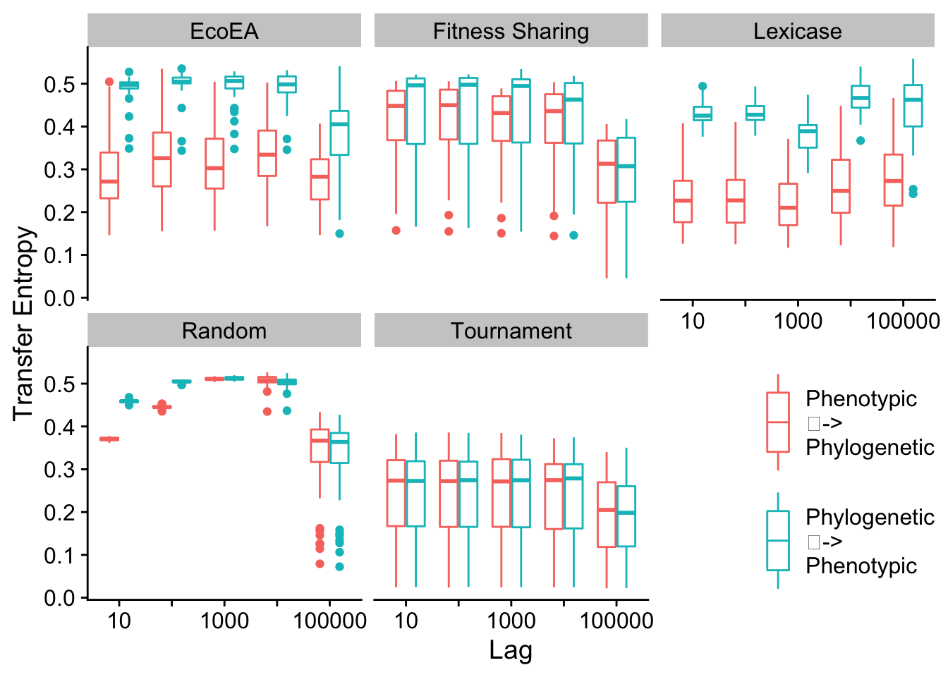

# Determine which conditions are significantly different from each other
transfer_entropy_stats(res)

selection_name	offset	.y.	group1	group2	n1	n2	statistic	p	p.adj	p.adj.signif	label	effsize	magnitude
EcoEA	10	value	Phenotypic -> Phylogenetic	Phylogenetic -> Phenotypic	50	50	101	0.00e+00	0.0000000	****	p < 1e-04	0.7920999	large
EcoEA	100	value	Phenotypic -> Phylogenetic	Phylogenetic -> Phenotypic	50	50	176	0.00e+00	0.0000000	****	p < 1e-04	0.7403963	large
EcoEA	1000	value	Phenotypic -> Phylogenetic	Phylogenetic -> Phenotypic	50	50	91	0.00e+00	0.0000000	****	p < 1e-04	0.7989937	large
EcoEA	10000	value	Phenotypic -> Phylogenetic	Phylogenetic -> Phenotypic	50	50	119	0.00e+00	0.0000000	****	p < 1e-04	0.7796910	large
EcoEA	100000	value	Phenotypic -> Phylogenetic	Phylogenetic -> Phenotypic	50	50	473	1.00e-07	0.0000022	****	p < 1e-04	0.5356498	large
Fitness Sharing	10	value	Phenotypic -> Phylogenetic	Phylogenetic -> Phenotypic	50	50	884	1.17e-02	0.2925000	ns	p = 0.2925	0.2523138	small
Fitness Sharing	100	value	Phenotypic -> Phylogenetic	Phylogenetic -> Phenotypic	50	50	905	1.76e-02	0.4400000	ns	p = 0.44	0.2378368	small
Fitness Sharing	1000	value	Phenotypic -> Phylogenetic	Phylogenetic -> Phenotypic	50	50	836	4.36e-03	0.1090000	ns	p = 0.109	0.2854041	small
Fitness Sharing	10000	value	Phenotypic -> Phylogenetic	Phylogenetic -> Phenotypic	50	50	994	7.82e-02	1.0000000	ns	p = 1	0.1764818	small
Fitness Sharing	100000	value	Phenotypic -> Phylogenetic	Phylogenetic -> Phenotypic	50	50	1247	9.86e-01	1.0000000	ns	p = 1	0.0020681	small
Lexicase	10	value	Phenotypic -> Phylogenetic	Phylogenetic -> Phenotypic	50	50	6	0.00e+00	0.0000000	****	p < 1e-04	0.8575912	large
Lexicase	100	value	Phenotypic -> Phylogenetic	Phylogenetic -> Phenotypic	50	50	9	0.00e+00	0.0000000	****	p < 1e-04	0.8555230	large
Lexicase	1000	value	Phenotypic -> Phylogenetic	Phylogenetic -> Phenotypic	50	50	44	0.00e+00	0.0000000	****	p < 1e-04	0.8313947	large
Lexicase	10000	value	Phenotypic -> Phylogenetic	Phylogenetic -> Phenotypic	50	50	24	0.00e+00	0.0000000	****	p < 1e-04	0.8451823	large
Lexicase	100000	value	Phenotypic -> Phylogenetic	Phylogenetic -> Phenotypic	50	50	195	0.00e+00	0.0000000	****	p < 1e-04	0.7272980	large
Random	10	value	Phenotypic -> Phylogenetic	Phylogenetic -> Phenotypic	50	50	0	0.00e+00	0.0000000	****	p < 1e-04	0.8617275	large
Random	100	value	Phenotypic -> Phylogenetic	Phylogenetic -> Phenotypic	50	50	0	0.00e+00	0.0000000	****	p < 1e-04	0.8617275	large
Random	1000	value	Phenotypic -> Phylogenetic	Phylogenetic -> Phenotypic	50	50	949	3.83e-02	0.9575000	ns	p = 0.9575	0.2075040	small
Random	10000	value	Phenotypic -> Phylogenetic	Phylogenetic -> Phenotypic	50	50	1558	3.40e-02	0.8500000	ns	p = 0.85	0.2123297	small
Random	100000	value	Phenotypic -> Phylogenetic	Phylogenetic -> Phenotypic	50	50	1304	7.12e-01	1.0000000	ns	p = 1	0.0372266	small
Tournament	10	value	Phenotypic -> Phylogenetic	Phylogenetic -> Phenotypic	50	50	1232	9.04e-01	1.0000000	ns	p = 1	0.0124089	small
Tournament	100	value	Phenotypic -> Phylogenetic	Phylogenetic -> Phenotypic	50	50	1261	9.42e-01	1.0000000	ns	p = 1	0.0075832	small
Tournament	1000	value	Phenotypic -> Phylogenetic	Phylogenetic -> Phenotypic	50	50	1252	9.92e-01	1.0000000	ns	p = 1	0.0013788	small
Tournament	10000	value	Phenotypic -> Phylogenetic	Phylogenetic -> Phenotypic	50	50	1217	8.23e-01	1.0000000	ns	p = 1	0.0227496	small
Tournament	100000	value	Phenotypic -> Phylogenetic	Phylogenetic -> Phenotypic	50	50	1240	9.48e-01	1.0000000	ns	p = 1	0.0068938	small

2.7.3.4 Mean evolutionary distinctiveness and phenotypic richness

res <- data %>% group_by(directory, selection_name) %>%
summarise(
  phen_phylo_10 =      condinformation(
                          discretize(phen_num_taxa), 
                          discretize(lag(mean_phenotype_evolutionary_distinctiveness, 1)), 
                          discretize(lag(phen_num_taxa, 1))),
  phen_phylo_100 =     condinformation(
                          discretize(phen_num_taxa),
                          discretize(lag(mean_phenotype_evolutionary_distinctiveness, 10)),
                          discretize(lag(phen_num_taxa, 10))),
  pheno_phylo_1000 =   condinformation(
                          discretize(phen_num_taxa),
                          discretize(lag(mean_phenotype_evolutionary_distinctiveness, 100)),
                          discretize(lag(phen_num_taxa, 100))),
  pheno_phylo_10000 =  condinformation(
                          discretize(phen_num_taxa),
                          discretize(lag(mean_phenotype_evolutionary_distinctiveness, 1000)),
                          discretize(lag(phen_num_taxa, 1000))),
  pheno_phylo_100000 = condinformation(
                          discretize(phen_num_taxa),
                          discretize(lag(mean_phenotype_evolutionary_distinctiveness, 10000)),
                          discretize(lag(phen_num_taxa, 10000))),
  
  phylo_pheno_10 =     condinformation(
                          discretize(mean_phenotype_evolutionary_distinctiveness),
                          discretize(lag(phen_num_taxa, 1)),
                          discretize(lag(mean_phenotype_evolutionary_distinctiveness, 1))),
  phylo_pheno_100 =    condinformation(
                          discretize(mean_phenotype_evolutionary_distinctiveness),
                          discretize(lag(phen_num_taxa, 10)),
                          discretize(lag(mean_phenotype_evolutionary_distinctiveness, 10))),
  phylo_pheno_1000 =   condinformation(
                          discretize(mean_phenotype_evolutionary_distinctiveness),
                          discretize(lag(phen_num_taxa, 100)),
                          discretize(lag(mean_phenotype_evolutionary_distinctiveness, 100))),
  phylo_pheno_10000 =  condinformation(
                          discretize(mean_phenotype_evolutionary_distinctiveness),
                          discretize(lag(phen_num_taxa, 1000)),
                          discretize(lag(mean_phenotype_evolutionary_distinctiveness, 1000))),
  phylo_pheno_100000 = condinformation(
                          discretize(mean_phenotype_evolutionary_distinctiveness),
                          discretize(lag(phen_num_taxa, 10000)),
                          discretize(lag(mean_phenotype_evolutionary_distinctiveness, 10000)))
)

# Turn Transfer Entropy columns into rows
res <- res %>% pivot_longer(cols=contains("phylo"))
# Pull lag into a column
res$offset <- str_extract(res$name, "[:digit:]*$")
# Make column indicating direction of transfer entropy
res$Type <- case_when(str_detect(res$name, "phylo_pheno") ~ "\nPhenotypic\n\t->\nPhylogenetic\n", TRUE ~ "\nPhylogenetic\n\t->\nPhenotypic\n")

ggplot(
  res, 
  aes(
    x=as.factor(offset), 
    y=value, 
    color=Type
    )
  ) + 
  geom_boxplot() + 
  facet_wrap(~selection_name) + 
  scale_x_discrete("Lag",labels=c("10","","1000","","100000")) + 
  scale_y_continuous("Transfer Entropy") + 
  theme(legend.position = c(1, 0),
        legend.justification = c(1, 0)) + 
  scale_color_discrete("")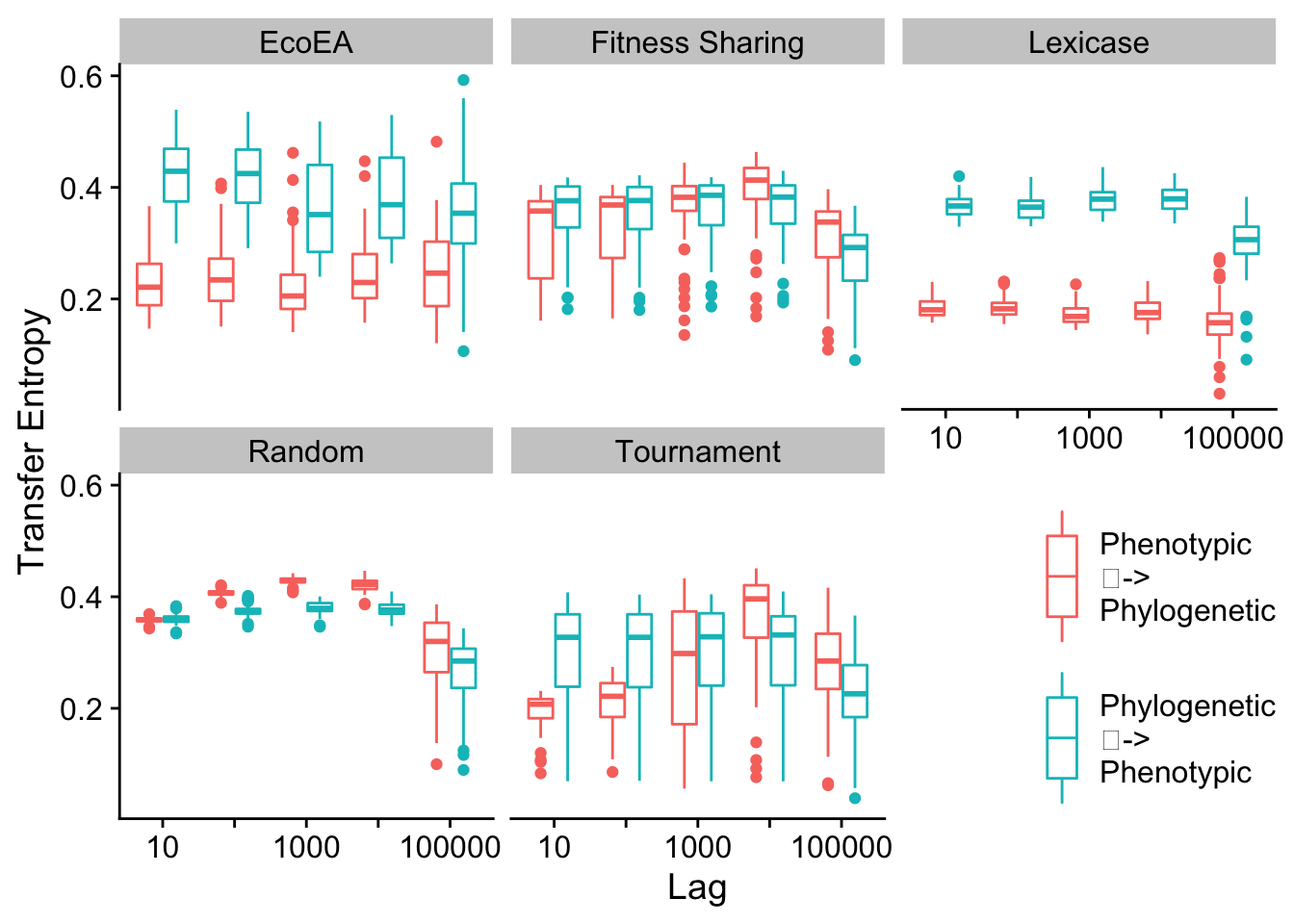

# Determine which conditions are significantly different from each other
transfer_entropy_stats(res)

selection_name	offset	.y.	group1	group2	n1	n2	statistic	p	p.adj	p.adj.signif	label	effsize	magnitude
EcoEA	10	value	Phenotypic -> Phylogenetic	Phylogenetic -> Phenotypic	50	50	25	0.00e+00	0.000000	****	p < 1e-04	0.8444929	large
EcoEA	100	value	Phenotypic -> Phylogenetic	Phylogenetic -> Phenotypic	50	50	96	0.00e+00	0.000000	****	p < 1e-04	0.7955468	large
EcoEA	1000	value	Phenotypic -> Phylogenetic	Phylogenetic -> Phenotypic	50	50	175	0.00e+00	0.000000	****	p < 1e-04	0.7410856	large
EcoEA	10000	value	Phenotypic -> Phylogenetic	Phylogenetic -> Phenotypic	50	50	216	0.00e+00	0.000000	****	p < 1e-04	0.7128210	large
EcoEA	100000	value	Phenotypic -> Phylogenetic	Phylogenetic -> Phenotypic	50	50	471	1.00e-07	0.000002	****	p < 1e-04	0.5370286	large
Fitness Sharing	10	value	Phenotypic -> Phylogenetic	Phylogenetic -> Phenotypic	50	50	817	2.87e-03	0.071750	ns	p = 0.07175	0.2985024	small
Fitness Sharing	100	value	Phenotypic -> Phylogenetic	Phylogenetic -> Phenotypic	50	50	946	3.64e-02	0.910000	ns	p = 0.91	0.2095721	small
Fitness Sharing	1000	value	Phenotypic -> Phylogenetic	Phylogenetic -> Phenotypic	50	50	1303	7.17e-01	1.000000	ns	p = 1	0.0365372	small
Fitness Sharing	10000	value	Phenotypic -> Phylogenetic	Phylogenetic -> Phenotypic	50	50	1795	1.74e-04	0.004350	**	p = 0.00435	0.3757132	moderate
Fitness Sharing	100000	value	Phenotypic -> Phylogenetic	Phylogenetic -> Phenotypic	50	50	1693	2.28e-03	0.057000	ns	p = 0.057	0.3053962	moderate
Lexicase	10	value	Phenotypic -> Phylogenetic	Phylogenetic -> Phenotypic	50	50	0	0.00e+00	0.000000	****	p < 1e-04	0.8617275	large
Lexicase	100	value	Phenotypic -> Phylogenetic	Phylogenetic -> Phenotypic	50	50	0	0.00e+00	0.000000	****	p < 1e-04	0.8617275	large
Lexicase	1000	value	Phenotypic -> Phylogenetic	Phylogenetic -> Phenotypic	50	50	0	0.00e+00	0.000000	****	p < 1e-04	0.8617275	large
Lexicase	10000	value	Phenotypic -> Phylogenetic	Phylogenetic -> Phenotypic	50	50	0	0.00e+00	0.000000	****	p < 1e-04	0.8617275	large
Lexicase	100000	value	Phenotypic -> Phylogenetic	Phylogenetic -> Phenotypic	50	50	154	0.00e+00	0.000000	****	p < 1e-04	0.7555627	large
Random	10	value	Phenotypic -> Phylogenetic	Phylogenetic -> Phenotypic	50	50	1159	5.33e-01	1.000000	ns	p = 1	0.0627338	small
Random	100	value	Phenotypic -> Phylogenetic	Phylogenetic -> Phenotypic	50	50	2482	0.00e+00	0.000000	****	p < 1e-04	0.8493186	large
Random	1000	value	Phenotypic -> Phylogenetic	Phylogenetic -> Phenotypic	50	50	2500	0.00e+00	0.000000	****	p < 1e-04	0.8617275	large
Random	10000	value	Phenotypic -> Phylogenetic	Phylogenetic -> Phenotypic	50	50	2474	0.00e+00	0.000000	****	p < 1e-04	0.8438036	large
Random	100000	value	Phenotypic -> Phylogenetic	Phylogenetic -> Phenotypic	50	50	1707	1.65e-03	0.041250		p = 0.04125	0.3150476	moderate
Tournament	10	value	Phenotypic -> Phylogenetic	Phylogenetic -> Phenotypic	50	50	356	0.00e+00	0.000000	****	p < 1e-04	0.6163075	large
Tournament	100	value	Phenotypic -> Phylogenetic	Phylogenetic -> Phenotypic	50	50	454	0.00e+00	0.000001	****	p < 1e-04	0.5487481	large
Tournament	1000	value	Phenotypic -> Phylogenetic	Phylogenetic -> Phenotypic	50	50	1154	5.10e-01	1.000000	ns	p = 1	0.0661807	small
Tournament	10000	value	Phenotypic -> Phylogenetic	Phylogenetic -> Phenotypic	50	50	1843	4.42e-05	0.001105	**	p = 0.001105	0.4088035	moderate
Tournament	100000	value	Phenotypic -> Phylogenetic	Phylogenetic -> Phenotypic	50	50	1736	8.17e-04	0.020425		p = 0.020425	0.3350396	moderate

2.7.3.5 Mean evolutionary distinctiveness and shannon diversity

res <- data %>% group_by(directory, selection_name) %>%
summarise(
  phen_phylo_10 =      condinformation(
                          discretize(phen_diversity), 
                          discretize(lag(mean_phenotype_evolutionary_distinctiveness, 1)), 
                          discretize(lag(phen_diversity, 1))),
  phen_phylo_100 =     condinformation(
                          discretize(phen_diversity),
                          discretize(lag(mean_phenotype_evolutionary_distinctiveness, 10)),
                          discretize(lag(phen_diversity, 10))),
  pheno_phylo_1000 =   condinformation(
                          discretize(phen_diversity),
                          discretize(lag(mean_phenotype_evolutionary_distinctiveness, 100)),
                          discretize(lag(phen_diversity, 100))),
  pheno_phylo_10000 =  condinformation(
                          discretize(phen_diversity),
                          discretize(lag(mean_phenotype_evolutionary_distinctiveness, 1000)),
                          discretize(lag(phen_diversity, 1000))),
  pheno_phylo_100000 = condinformation(
                          discretize(phen_diversity),
                          discretize(lag(mean_phenotype_evolutionary_distinctiveness, 10000)),
                          discretize(lag(phen_diversity, 10000))),
  
  phylo_pheno_10 =     condinformation(
                          discretize(mean_phenotype_evolutionary_distinctiveness),
                          discretize(lag(phen_diversity, 1)),
                          discretize(lag(mean_phenotype_evolutionary_distinctiveness, 1))),
  phylo_pheno_100 =    condinformation(
                          discretize(mean_phenotype_evolutionary_distinctiveness),
                          discretize(lag(phen_diversity, 10)),
                          discretize(lag(mean_phenotype_evolutionary_distinctiveness, 10))),
  phylo_pheno_1000 =   condinformation(
                          discretize(mean_phenotype_evolutionary_distinctiveness),
                          discretize(lag(phen_diversity, 100)),
                          discretize(lag(mean_phenotype_evolutionary_distinctiveness, 100))),
  phylo_pheno_10000 =  condinformation(
                          discretize(mean_phenotype_evolutionary_distinctiveness),
                          discretize(lag(phen_diversity, 1000)),
                          discretize(lag(mean_phenotype_evolutionary_distinctiveness, 1000))),
  phylo_pheno_100000 = condinformation(
                          discretize(mean_phenotype_evolutionary_distinctiveness),
                          discretize(lag(phen_diversity, 10000)),
                          discretize(lag(mean_phenotype_evolutionary_distinctiveness, 10000)))
)

# Turn Transfer Entropy columns into rows
res <- res %>% pivot_longer(cols=contains("phylo"))
# Pull lag into a column
res$offset <- str_extract(res$name, "[:digit:]*$")
# Make column indicating direction of transfer entropy
res$Type <- case_when(str_detect(res$name, "phylo_pheno") ~ "\nPhenotypic\n\t->\nPhylogenetic\n", TRUE ~ "\nPhylogenetic\n\t->\nPhenotypic\n")

ggplot(
  res, 
  aes(
    x=as.factor(offset), 
    y=value, 
    color=Type
    )
  ) + 
  geom_boxplot() + 
  facet_wrap(~selection_name) + 
  scale_x_discrete("Lag",labels=c("10","","1000","","100000")) + 
  scale_y_continuous("Transfer Entropy") + 
  theme(legend.position = c(1, 0),
        legend.justification = c(1, 0)) + 
  scale_color_discrete("")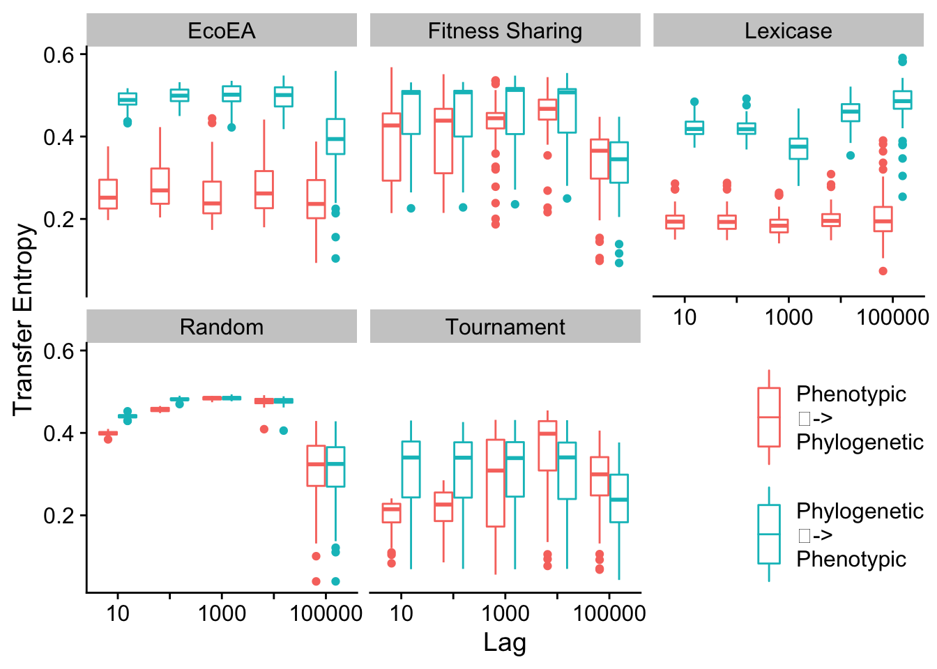

# Determine which conditions are significantly different from each other
transfer_entropy_stats(res)

selection_name	offset	.y.	group1	group2	n1	n2	statistic	p	p.adj	p.adj.signif	label	effsize	magnitude
EcoEA	10	value	Phenotypic -> Phylogenetic	Phylogenetic -> Phenotypic	50	50	0	0.00e+00	0.0000000	****	p < 1e-04	0.8617275	large
EcoEA	100	value	Phenotypic -> Phylogenetic	Phylogenetic -> Phenotypic	50	50	0	0.00e+00	0.0000000	****	p < 1e-04	0.8617275	large
EcoEA	1000	value	Phenotypic -> Phylogenetic	Phylogenetic -> Phenotypic	50	50	5	0.00e+00	0.0000000	****	p < 1e-04	0.8582806	large
EcoEA	10000	value	Phenotypic -> Phylogenetic	Phylogenetic -> Phenotypic	50	50	2	0.00e+00	0.0000000	****	p < 1e-04	0.8603487	large
EcoEA	100000	value	Phenotypic -> Phylogenetic	Phylogenetic -> Phenotypic	50	50	289	0.00e+00	0.0000000	****	p < 1e-04	0.6624961	large
Fitness Sharing	10	value	Phenotypic -> Phylogenetic	Phylogenetic -> Phenotypic	50	50	768	9.02e-04	0.0225500		p = 0.02255	0.3322821	moderate
Fitness Sharing	100	value	Phenotypic -> Phylogenetic	Phylogenetic -> Phenotypic	50	50	762	7.77e-04	0.0194250		p = 0.019425	0.3364184	moderate
Fitness Sharing	1000	value	Phenotypic -> Phylogenetic	Phylogenetic -> Phenotypic	50	50	809	2.39e-03	0.0597500	ns	p = 0.05975	0.3040175	moderate
Fitness Sharing	10000	value	Phenotypic -> Phylogenetic	Phylogenetic -> Phenotypic	50	50	988	7.14e-02	1.0000000	ns	p = 1	0.1806181	small
Fitness Sharing	100000	value	Phenotypic -> Phylogenetic	Phylogenetic -> Phenotypic	50	50	1312	6.72e-01	1.0000000	ns	p = 1	0.0427417	small
Lexicase	10	value	Phenotypic -> Phylogenetic	Phylogenetic -> Phenotypic	50	50	0	0.00e+00	0.0000000	****	p < 1e-04	0.8617275	large
Lexicase	100	value	Phenotypic -> Phylogenetic	Phylogenetic -> Phenotypic	50	50	0	0.00e+00	0.0000000	****	p < 1e-04	0.8617275	large
Lexicase	1000	value	Phenotypic -> Phylogenetic	Phylogenetic -> Phenotypic	50	50	0	0.00e+00	0.0000000	****	p < 1e-04	0.8617275	large
Lexicase	10000	value	Phenotypic -> Phylogenetic	Phylogenetic -> Phenotypic	50	50	0	0.00e+00	0.0000000	****	p < 1e-04	0.8617275	large
Lexicase	100000	value	Phenotypic -> Phylogenetic	Phylogenetic -> Phenotypic	50	50	23	0.00e+00	0.0000000	****	p < 1e-04	0.8458717	large
Random	10	value	Phenotypic -> Phylogenetic	Phylogenetic -> Phenotypic	50	50	0	0.00e+00	0.0000000	****	p < 1e-04	0.8617275	large
Random	100	value	Phenotypic -> Phylogenetic	Phylogenetic -> Phenotypic	50	50	0	0.00e+00	0.0000000	****	p < 1e-04	0.8617275	large
Random	1000	value	Phenotypic -> Phylogenetic	Phylogenetic -> Phenotypic	50	50	1208	7.75e-01	1.0000000	ns	p = 1	0.0289540	small
Random	10000	value	Phenotypic -> Phylogenetic	Phylogenetic -> Phenotypic	50	50	1244	9.70e-01	1.0000000	ns	p = 1	0.0041363	small
Random	100000	value	Phenotypic -> Phylogenetic	Phylogenetic -> Phenotypic	50	50	1257	9.64e-01	1.0000000	ns	p = 1	0.0048257	small
Tournament	10	value	Phenotypic -> Phylogenetic	Phylogenetic -> Phenotypic	50	50	394	0.00e+00	0.0000001	****	p < 1e-04	0.5901110	large
Tournament	100	value	Phenotypic -> Phylogenetic	Phylogenetic -> Phenotypic	50	50	482	1.00e-07	0.0000030	****	p < 1e-04	0.5294454	large
Tournament	1000	value	Phenotypic -> Phylogenetic	Phylogenetic -> Phenotypic	50	50	1107	3.26e-01	1.0000000	ns	p = 1	0.0985816	small
Tournament	10000	value	Phenotypic -> Phylogenetic	Phylogenetic -> Phenotypic	50	50	1739	7.58e-04	0.0189500		p = 0.01895	0.3371078	moderate
Tournament	100000	value	Phenotypic -> Phylogenetic	Phylogenetic -> Phenotypic	50	50	1675	3.43e-03	0.0857500	ns	p = 0.08575	0.2929873	small

References

Allen, Micah, Davide Poggiali, Kirstie Whitaker, Tom Rhys Marshall, Jordy van Langen, and Rogier A. Kievit. 2021. “Raincloud Plots: A Multi-Platform Tool for Robust Data Visualization.” Wellcome Open Research 4 (January): 63. https://doi.org/10/ghvbc6.

Hernandez, Jose Guadalupe, Alexander Lalejini, and Charles Ofria. 2021. “An Exploration of Exploration: Measuring the Ability of Lexicase Selection to Find Obscure Pathways to Optimality.” arXiv:2107.09760 [Cs], July. http://arxiv.org/abs/2107.09760.